Diffusion Models and Flow Matching

by Xiaolei Chu, Ph.D. candidate @ UC Berkeley

Part A.0: Setup

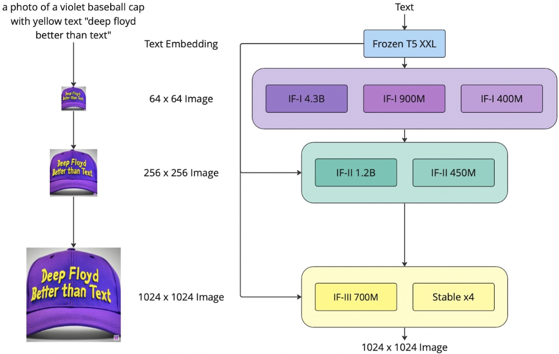
In this demo, we will use the DeepFloyd IF diffusion model, which is a two stage model trained by Stability AI. The first stage produces images of size \(64 \times 64\) and the second stage can make the \(64 \times 64\) be larger, \(256 \times 256\). The recent version also has a third stage, which can make higher resolution. DeepFloyd was trained as a text-to-image model, which takes text prompts as input and outputs images that are aligned with the text. We choose T5 as the text encoder to generate embeddings for the prompt. Throughout this demo, the random seed is always \(666\) for everything, i.e., torch.cuda.manual_seed(666), torch.manual_seed(666), and random.seed(666). The framework is shown in Figure 1.

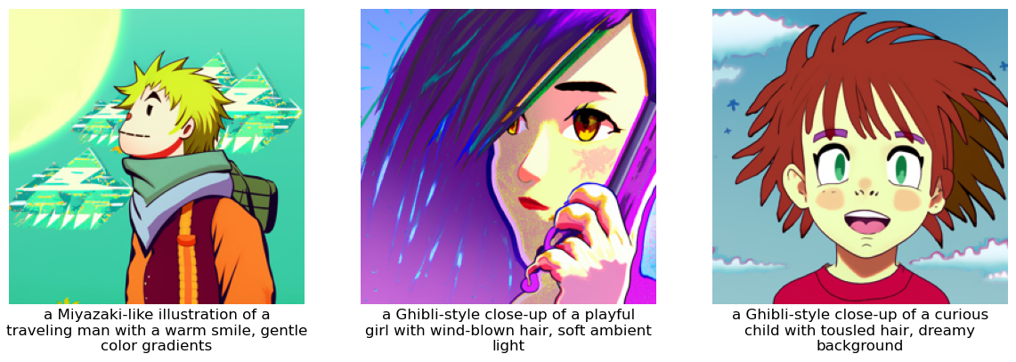
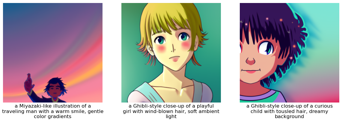
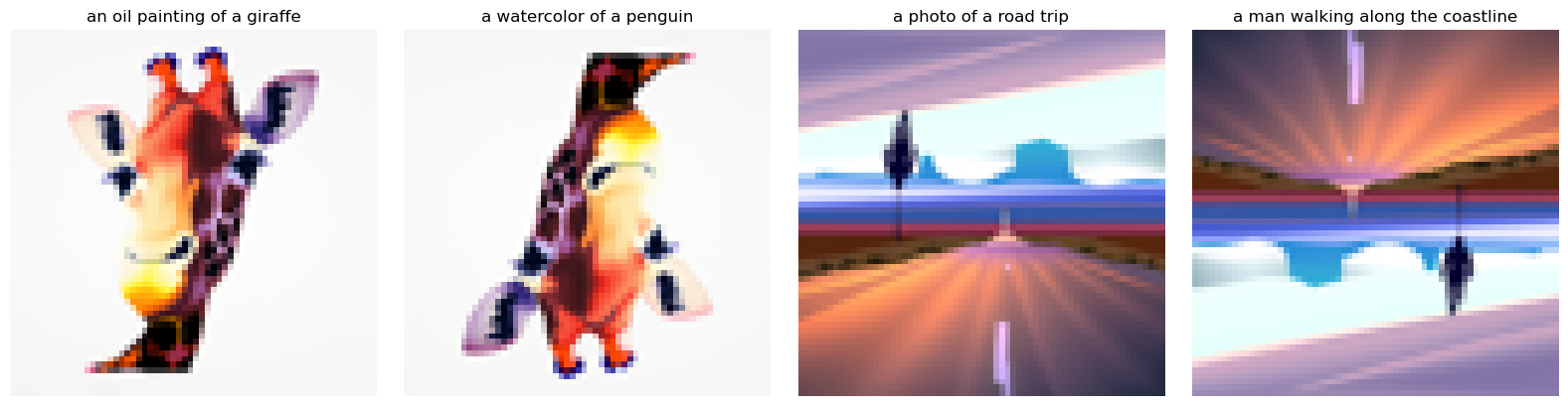
Let's try different text prompts (each embedding has shape \([1, 77, 4096]\), i.e., \([\text{batch}, \text{max_seq_len}, \text{embed_dim}]\)), embeddings of which are generated by T5 encoder. The generated with different inference steps are shown in Figure 2 and Figure 3, respectively.

Summaries

• The random seed is chosen as \(666\);
• According to Figure 2 and Figure 3, we can find different inference steps lead to images of different qualities. We notice that more steps can lead to sharper details, more stable structure, better alignment with the prompt, and reduced noise and artifacts.
• The prompts are:
  • a Miyazaki-like illustration of a traveling man with a warm smile, gentle color gradients;
  • a Ghibli-style close-up of a playful girl with wind-blown hair, soft ambient light;
  • a Ghibli-style close-up of a curious child with tousled hair, dreamy background.

Part A.1: Sampling Loops

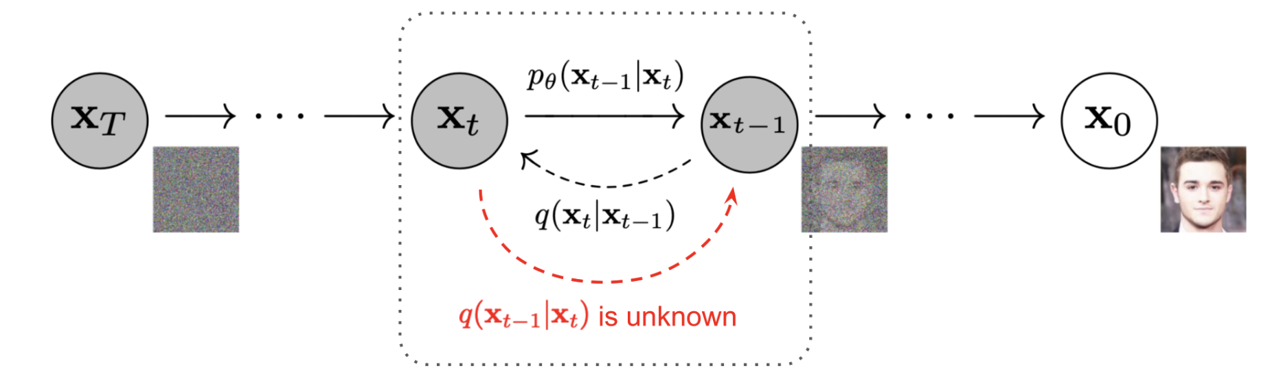
Starting with a clean image, \(x_0\), we can iteratively add noise to an image, obtaining progressively more and more noisy version of the image, \(x_t\), until we are left with basically pure noise at timestep \(t=T\). For the DeepFloyd models, \(T=1000\). A diffusion model tries to reverse this process by denoising the image. Briefly, a diffusion model tries to predict the noise in the image given a noisy \(x_t\) and the timestep \(t\). The whole process is shown in Figure 4.

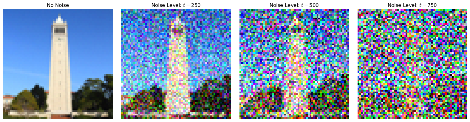
1.1 Implementing the Forward Process

A key part of difussion is the forward process, which takes a clean image and adds noise to it. The forward process is defined by:

The forward process is demonstrated in Figure 5.

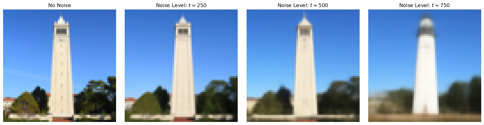
1.2 Classical Denoising

As a comparison with the diffusion, we first try to denoise these noisy images using classical methods, e.g., Gaussian blur filtering. We use torchvision.transforms.functional.gaussian_blur to denoise images. The Gaussian-denoised version is shown in Figure 6.

1.3 Implementing One Step Denoising

From Figure 6, we know the classical denoising methods cannot work well. Thus, we will use a pretrained diffusion model to denoise. The denoiser that we use is stage_1.unet, which is a UNet that has already been trained on a very, very large dataset of \(\left(x_0, x_t\right)\) pairs of images. We can use it to recover Gaussian noise from the image. Then, we can remove this noise to recover (something close to) the original image. The one-step denoising effect can be found in Figure 7. We can notice that the pretrained diffusion model performs much better than the Gaussian blur filters. When the noise level is low, the diffusion model can nearly completely recover the image. When the noise level is high, the diffusion model can still recover the general feature of the image, but in which the higher frequency information is mostly lost.

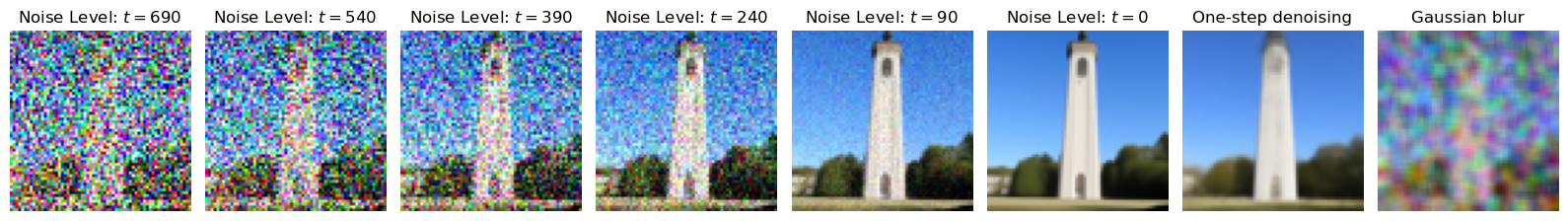
1.4 Implementing Iterative Denoising

Iterative denoising means that we do not denoise the image using only one step. Instead, we iteratively recover the noisy image to the less noisy one, and finally we recover the original image. To actually do this, we have the following formula:

• \(x_t\) is the image at timestep \(t\);
• \(x_{t^\prime}\) is the noisy image at timestep \(t^\prime\) where \(t^\prime < t\) (less noisy);
• \(\bar{\alpha}_t\) is defined by alphas_cumprod, which is stored in stage_1.unet.
• \(\alpha_t = \bar{\alpha}_t / \bar{\alpha}_{t^\prime}\)
• \(\beta_t = 1 - \alpha_t\)
• \(x_0\) is our current estimate of the clean image.

We implement the iterative denoising, as shown in Figure 8. Compared with the one-step denoising, we can find that there are more sharper characters. Again, the Gaussian blur cannot recover the image.

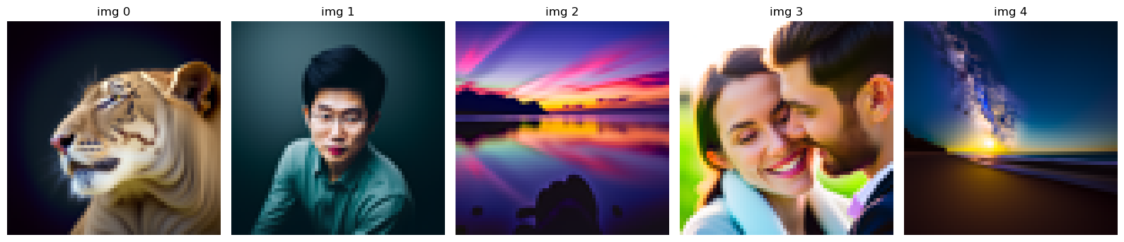
1.5 Diffusion Model Sampling

In this part, we want the diffusion model to denoise an image that is purely random noise. Since the DeepFloyd model is prompt-based, the prompt we use here is "a high quality photo". The generated images are shown in Figure 9. We can still tell the objects from the images, though the quality is not good.

1.6 Classifier-Free Guidance

We can notice that the generated images in the prior section are not very good. In order to greatly improve image quality (at the expense of image diversity), we can use a technique called Classifier-Free Guidance (CFG). In CFG, we compute both a conditional and an unconditonal noise estimate. We denote these \(\epsilon_{c}\) and \(\epsilon_{u}\). Then, we let our new noise estimate be:

Using the CFG, the denoised images are shown in Figure 10, which are much better.

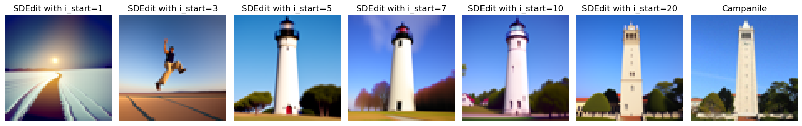
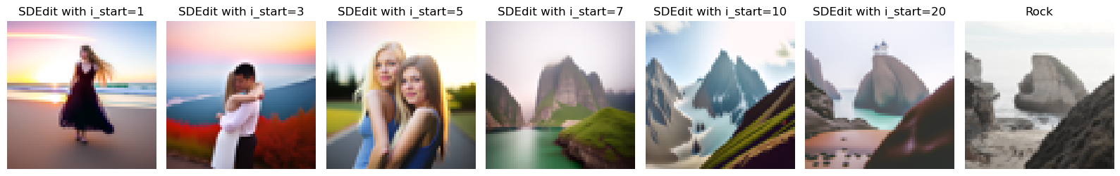
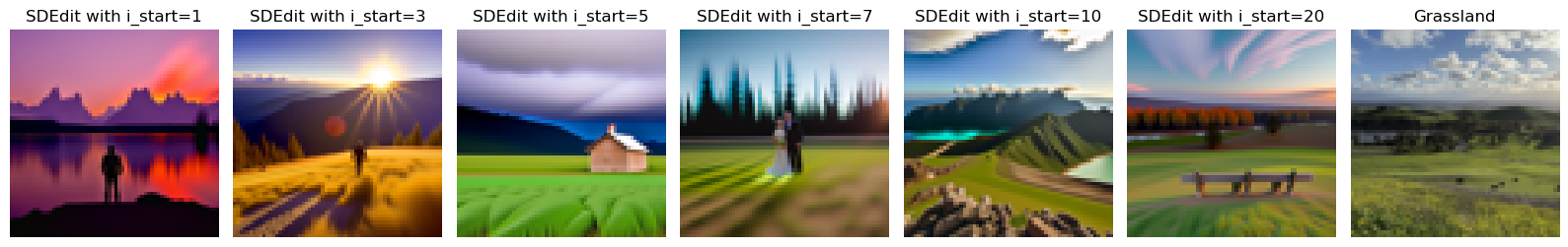
1.7 Image-to-image Translation

Here, we are going to take some original images, noise them a little, and force them back onto the image manifold without any conditioning. This follows the SDEdit algorithm. Again, we use "a high quality photo" as the conditonal text prompt.

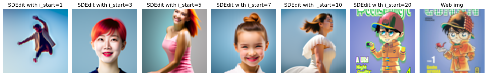
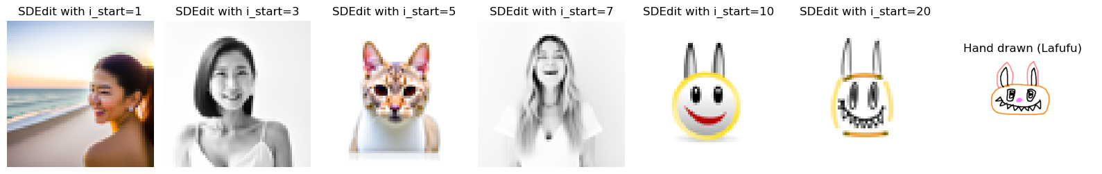
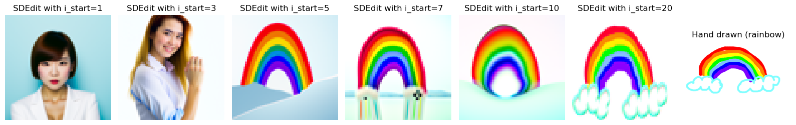
1.7.1 Editing Hand-Drawn and Web Images

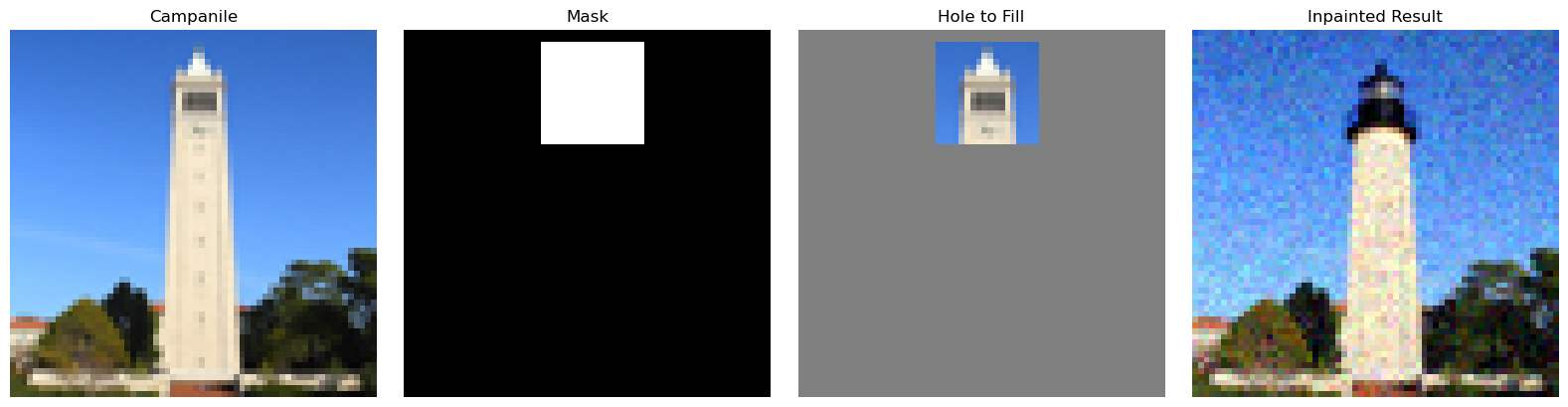
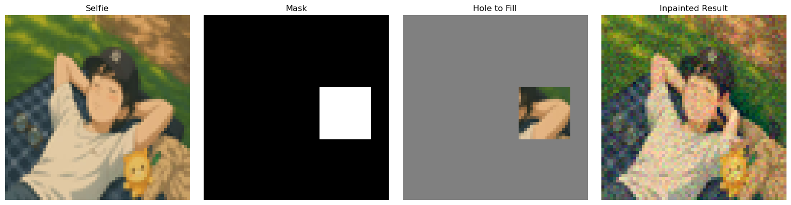
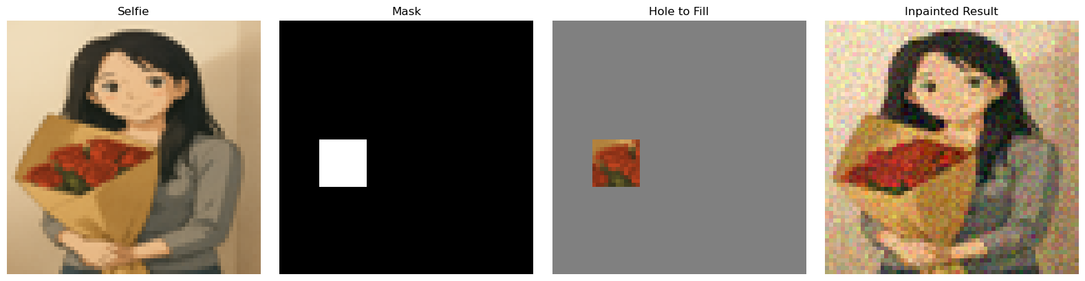
1.7.2 Inpainting

We can use the same procedure to implement inpainting (following the RePaint paper). That is, given an image \(x_{\text{orig}}\) and a binary mask \(\mathbf{m}\), we can create a new image that has the same content where \(\mathbf{m}\) is 0, but new content wherever \(\mathbf{m}\) is 1. To do this, we can run the diffusion denoising loop. But at every step, after obtaining \(x_{t}\), we "force" \(x_t\) to have the same pixels as \(x_{\text{orig}}\) where \(\mathbf{m}\) is 0, i.e.,

Essentially, we leave everything inside the edit mask alone, but we replace everything outside the edit mask with our original image -- with the correct amount of noise added for timestep \(t\). We try three different images, as shown below.

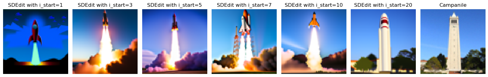
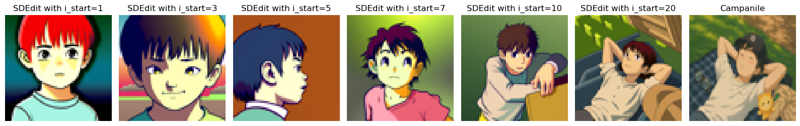
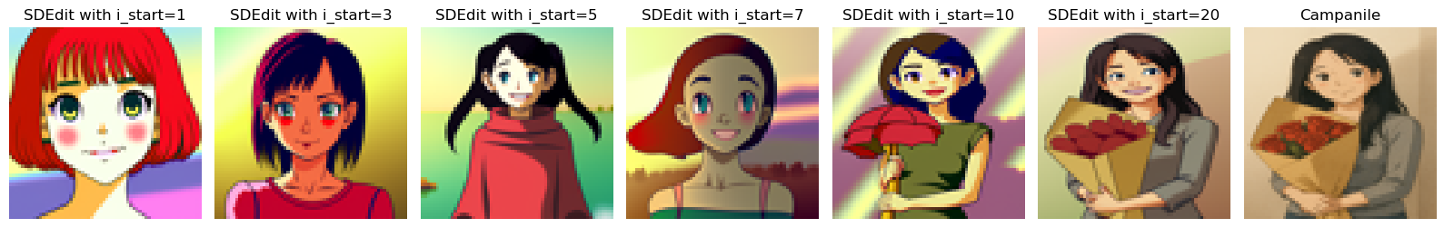
1.7.3 Text-Conditional Image-to-image Translation

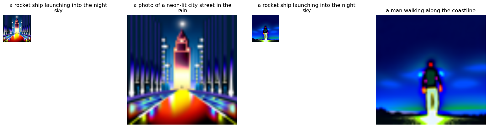
Now, we will do the same thing as SDEdit, but guide the projection with a text prompt. We try three different images, as shown below.

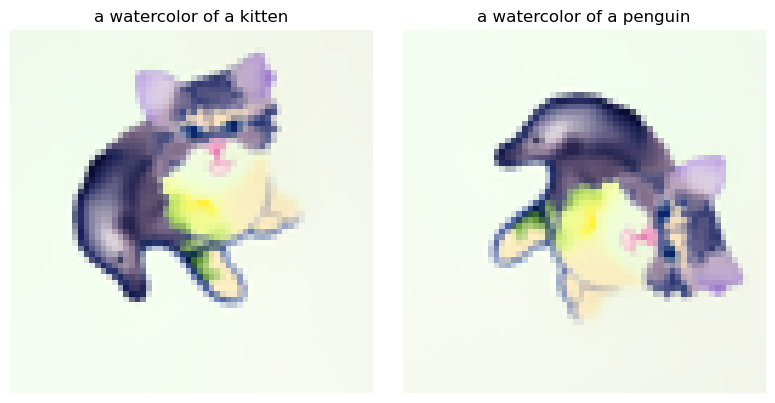
1.8 Visual Anagrams

We will implement Visual Anagrams and create optical illusions with diffusion models. In this part, we will create an image that looks differently when flipped upside down.

To do this, we will denoise an image \(x_t\) at step \(t\) normally with the prompt \(p_1\), to obtain noise estimate \(\epsilon_1\). But at the same time, we will flip \(x_t\) upside down, and denoise with the prompt \(p_2\), to get noise estimate \(\epsilon_2\). We can flip \(\epsilon_2\) back, and average the two noise estimates. We can then perform a reverse/denoising diffusion step with the averaged noise estimate. The full algorithm will be:

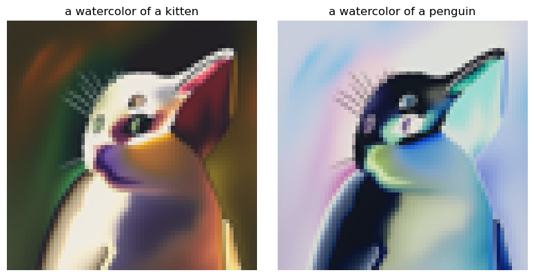
1.9 Hybrid Images

We will implement Factorized Diffusion and create hybrid images. In order to create hybrid images with a diffusion model we can use a similar technique as above. We will create a composite noise estimate \(\epsilon\), by estimating the noise with two different text prompts, and then combining low frequencies from one noise estimate with high frequencies of the other. The algorithm is:

Part A.2: Bells & Whistles

More visual anagrams!

We will implement another two visual anagrams, \(90^\circ\) rotations and color inversions.

For \(90^\circ\) rotations, the algorithm follows:

For color inversions, the algorithm follows:

Design a course logo!

Part B.1: Training a Single-Step Denoising UNet

In this part, we will focus on training our own Flow Matching model on MNIST dataset. We choose the UNet model as the backbone and build it from scratch.

1.0 Recap of Flow Matching for Generative Modeling

Flow matching is a method for training continuous-time generative models by directly learning a probability flow that transports a simple base distribution to a complex data distribution. Instead of using stochastic diffusion processes, flow matching learns a deterministic ordinary differential equation (ODE) whose solution maps base samples to data samples.

Let \( p_0(x) \) be a simple base distribution (e.g. standard Gaussian) and \( p_1(x) \) be the data distribution. Flow matching introduces a time-dependent family of intermediate distributions \( p_t(x) \), for \( t \in [0, 1] \), that smoothly connects them:

The evolution of samples over time is described by an ODE:

where \( v_\theta(t, x) \) is a neural network (the velocity field) with parameters \( \theta \). This ODE induces a probability flow that pushes forward \( p_0 \) into \( p_1 \).

The time evolution of the distributions \( p_t(x) \) under the flow is governed by the continuity equation:

Flow matching assumes we can construct a probability path \( p_t(x) \) between \( p_0 \) and \( p_1 \), for which there exists an oracle or analytically defined vector field \( u_t(x) \) such that:

There are a lot of ways to construct the vector field. What we use here is a simple but useful one, coupling base and data samples via a simple interpolation, a.k.a. rectified flow. Sample \( x_0 \sim p_0 \), \( x_1 \sim p_1 \), and define an interpolated state:

The corresponding oracle velocity along this path is:

In practice, we can sample triples \( (x_0, x_1, t) \), compute \( x_t \), and treat \( (x_t, t) \) as inputs and \( u_t(x_t) = x_1 - x_0 \) as the regression target for the model \( v_\theta \).

The flow matching objective is typically a mean-squared error between the learned velocity field and the oracle velocity:

Minimizing \( \mathcal{L}(\theta) \) encourages the learned flow to follow the same probability evolution as the designed path \( p_t \).

After training, generative sampling proceeds by:

1. Sampling \( x_0 \sim p_0(x) \) (e.g. Gaussian noise).
2. Solving the ODE forward in time:
   \( \frac{d x_t}{d t} = v_\theta(t, x_t), \quad t \in [0, 1], \quad x_{t=0} = x_0. \)
3. Taking \( x_{t=1} \) as a generated sample from an approximation of \( p_1(x) \).

Flow matching can be seen as a deterministic counterpart to diffusion-based generative modeling. Diffusion models learn a score function for a noisy stochastic process and often require reverse-time SDE or ODE solvers. In contrast, flow matching directly learns a deterministic velocity field that transports probability mass, avoiding stochastic perturbations during training and sampling.

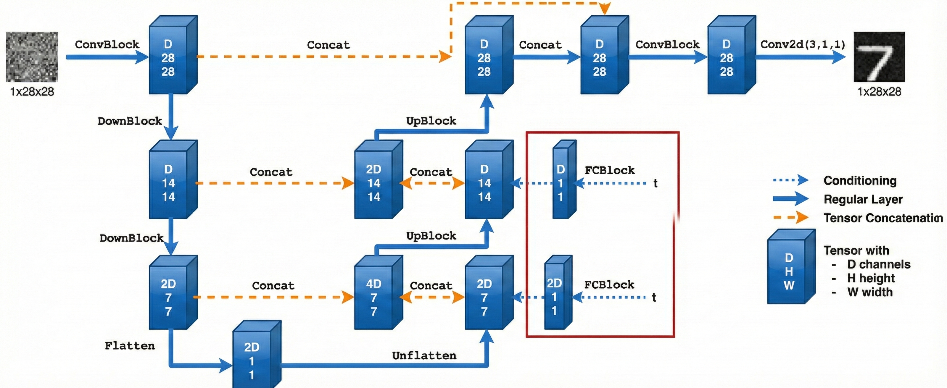
1.1 Implementing the UNet

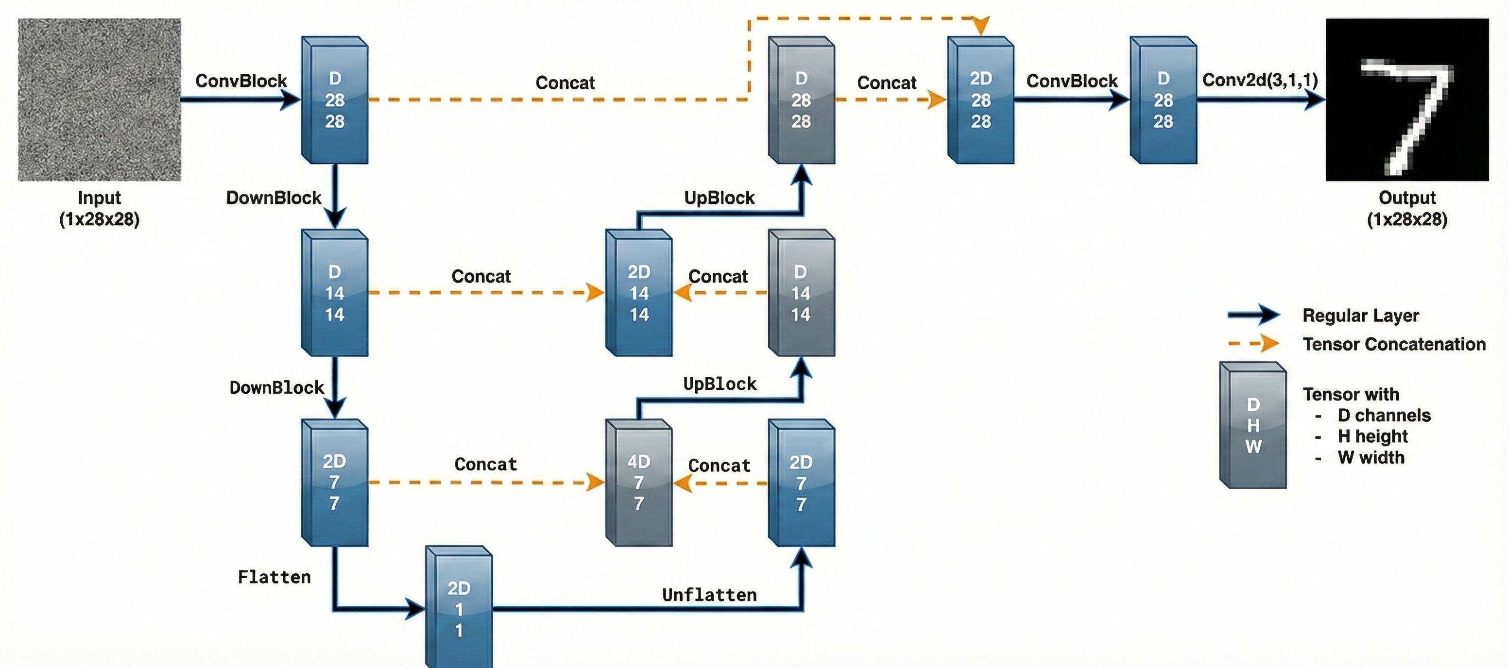
We implement the denoiser as a UNet, which consists of a few downsampling and upsampling blocks with skip connections. Specifically, the architecture is shown in Figure 28.

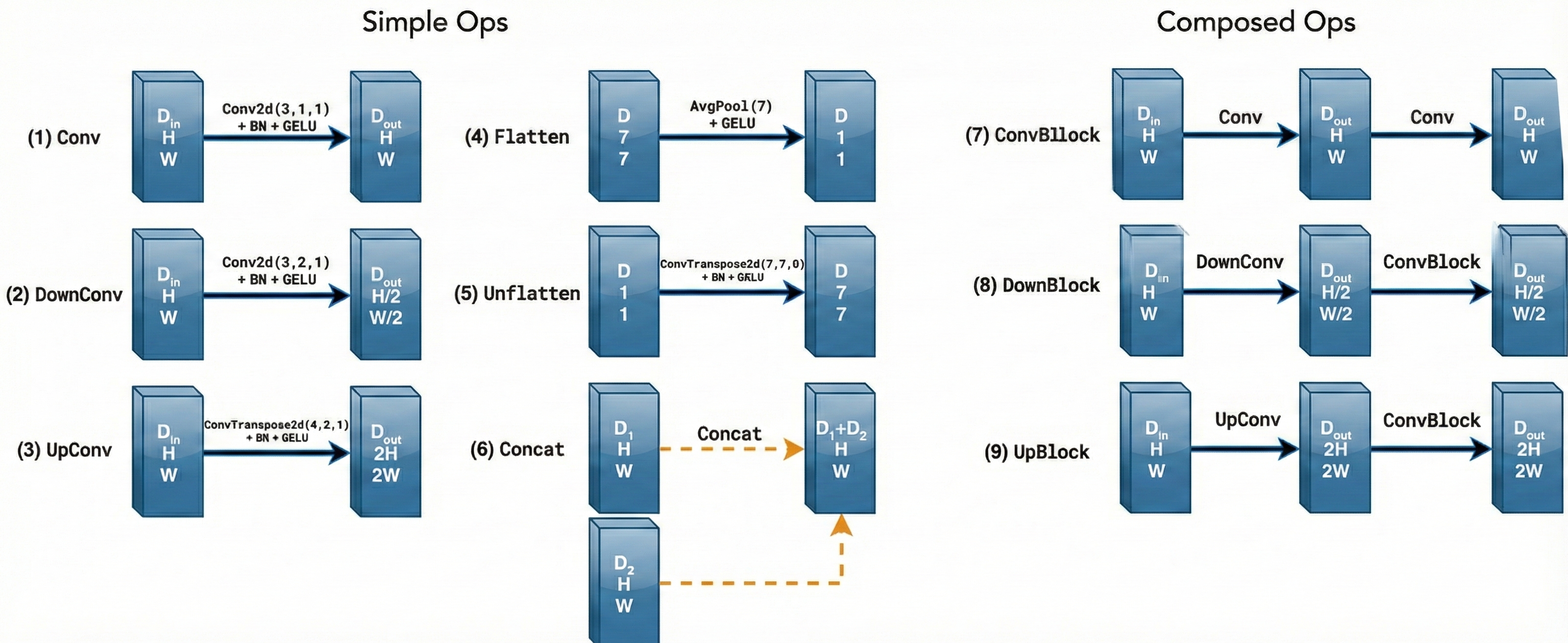
The diagram above uses a number of standard tensor operations defined as follows:

1.2 Using the UNet to Train a Denoiser

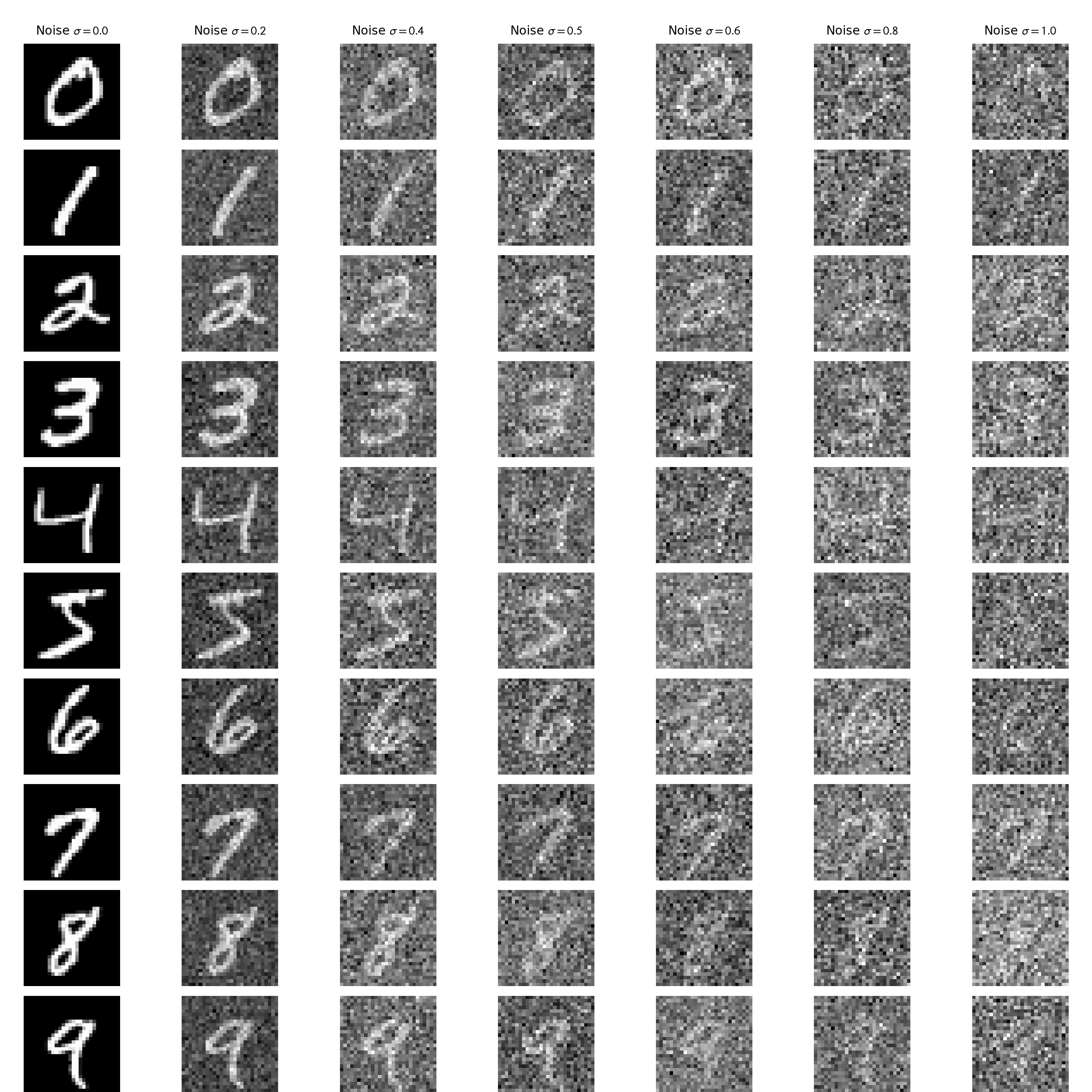
For now, we focus on the simpler problem, i.e., one-step denoising. To train our denoiser, we need to generate training data pairs of \((z,x)\), where each \(x\) is a clean MNIST digit. For each training batch, we can generate \(z\) from \(x\) using the following noising process:

where \(\sigma\) controls the noise level. As shown in Figure 30, the images are contaminated with noise at different intensities, each determined by a specific \(\sigma\) value.

1.2.1 Training

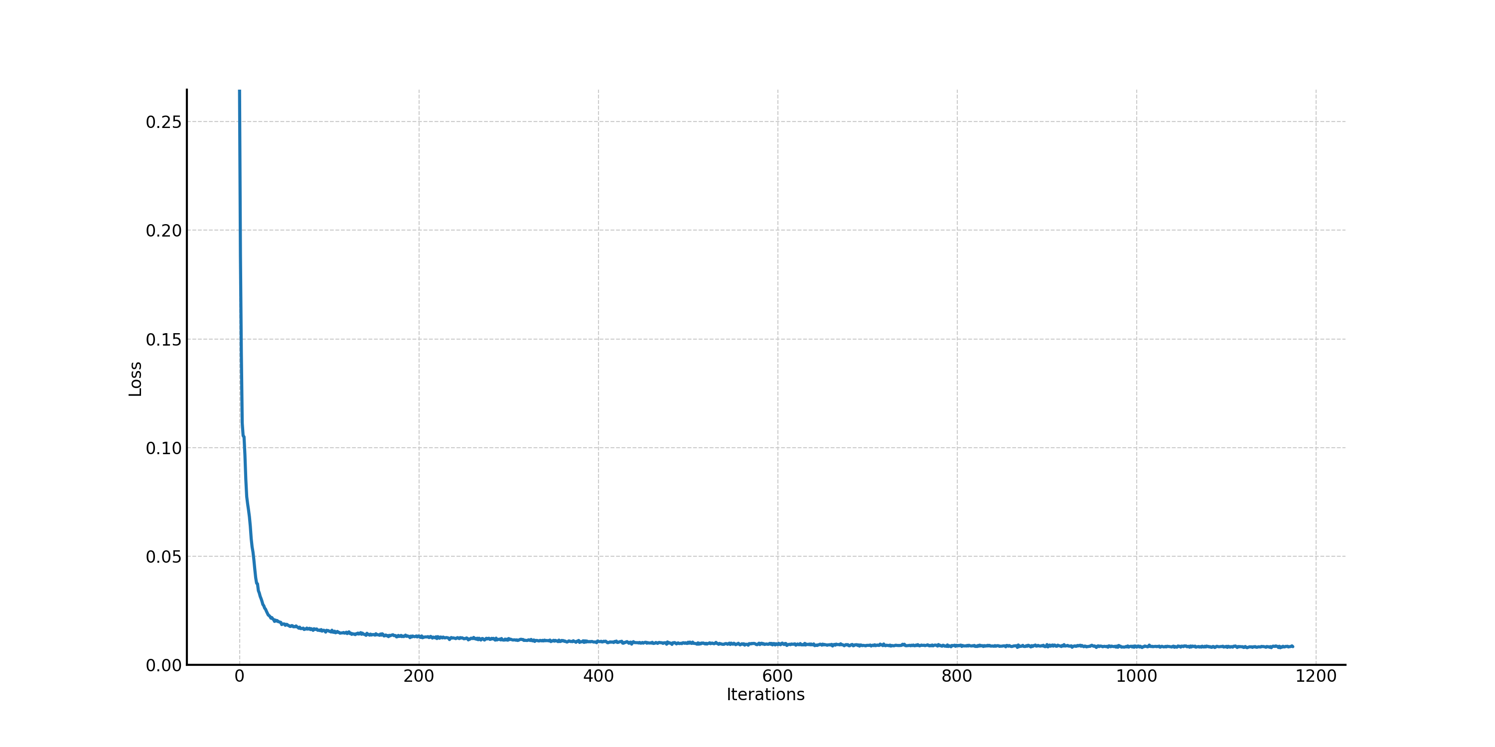
Now we train this denoiser to denoise noisy image \(z\) with \(\sigma=0.5\) applied to a clean image \(x\), which means other \(\sigma\) values are out-of-distribution testing cases. The configuration of this one-step denoising model is shown in Table 1. The procedure of the training loss is shown in Figure 31. You can expand the following unconditional UNet architecture block to see the details.

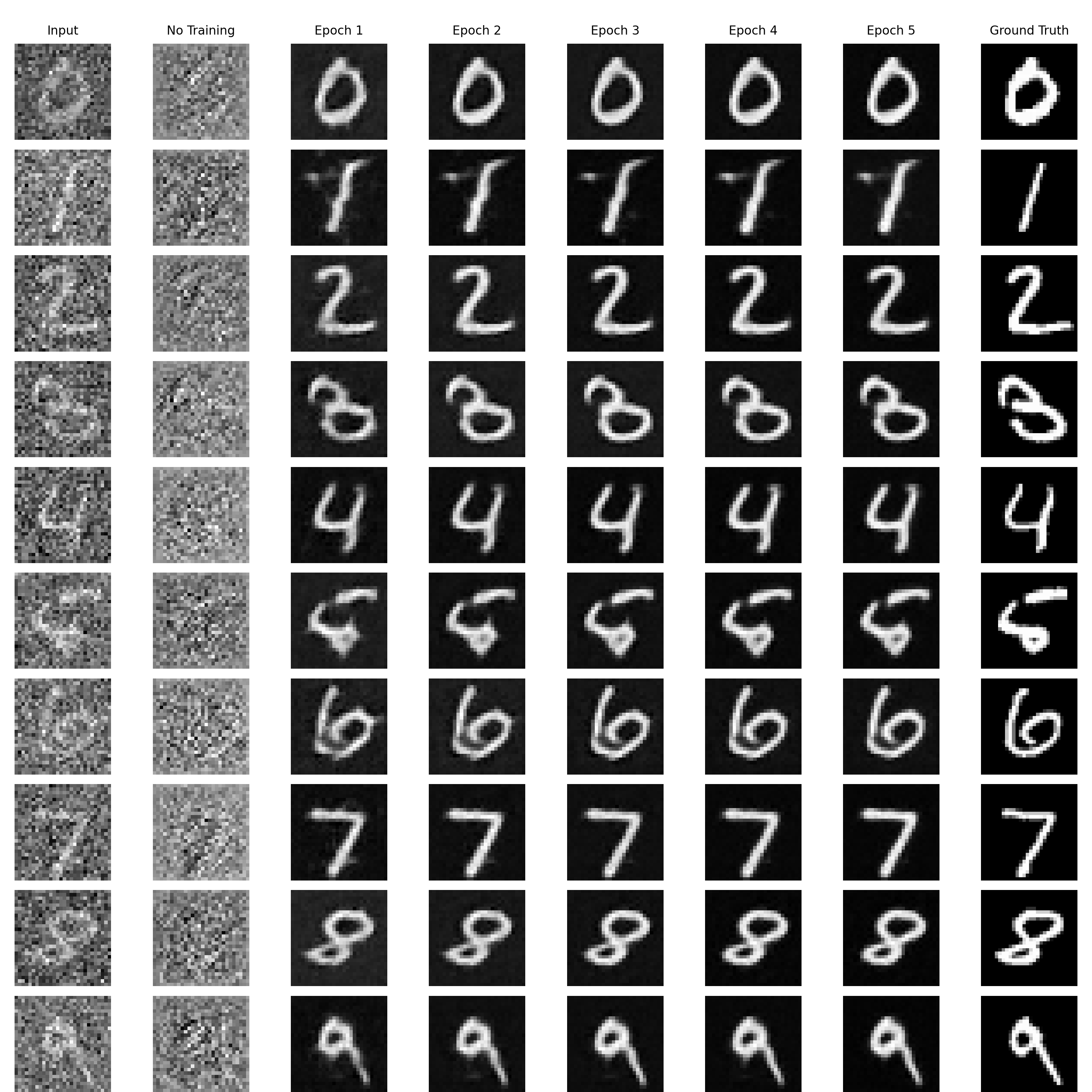
With the noise level \(\sigma = 0.5\), we sample results on the test set to see if the one-step denoising UNet can work. In Figure 32, we can find that noise level 0.5 is kind of large because, for example, it is hard for people to tell the noisy input with the digit "5". The convergence is very fast so that even with one epoch training, the denoising effect is satisfactory. After 5 epoch training, the results look very good.

1.2.2 Out-of-Distribution Testing

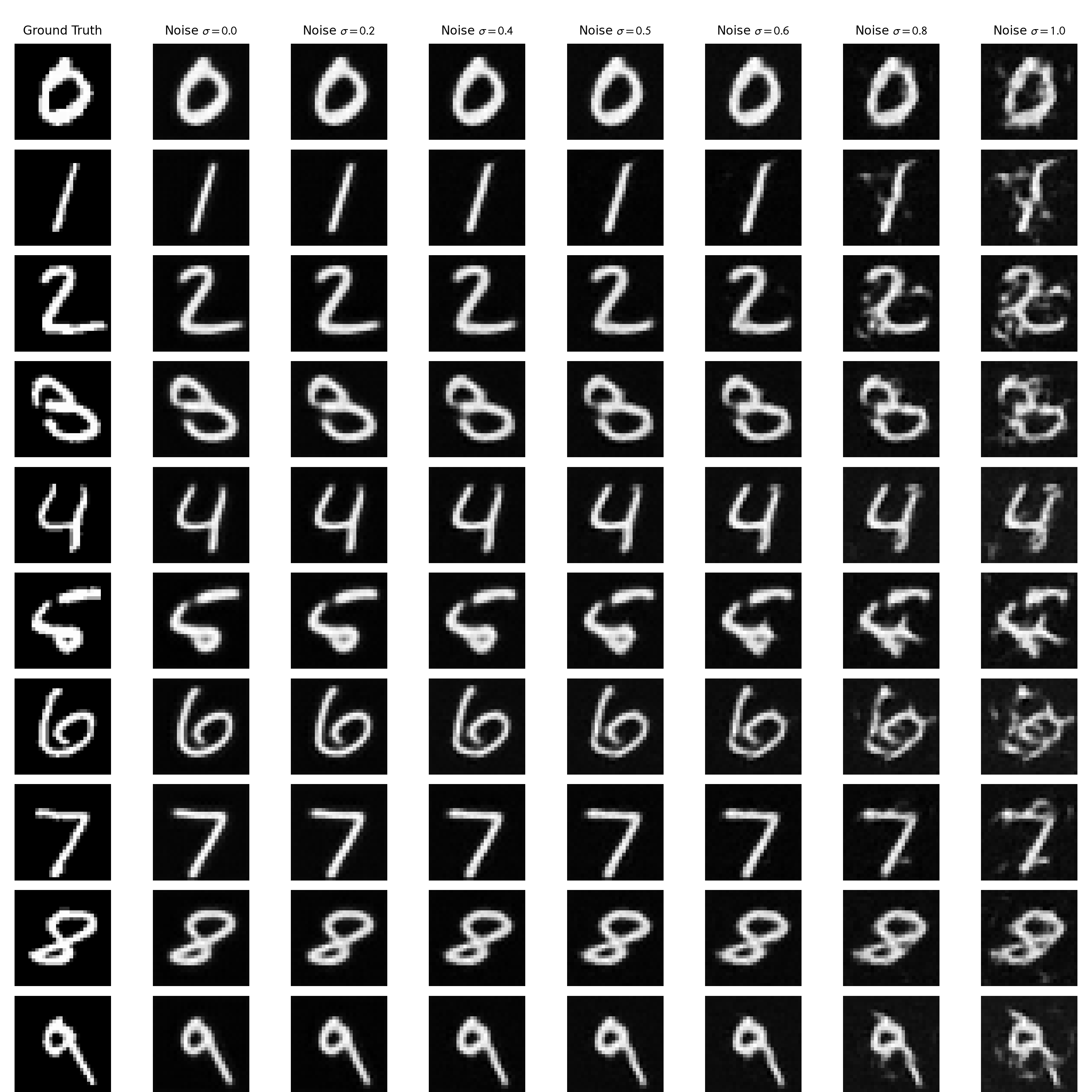
Our one-step denoiser was trained with \(\sigma = 0.5\). Now let's examine its out-of-distribution capacity. We vary the levels of noise to see if the one-step denoiser still works. In Figure 33, we can notice when the noise is not large (\(\sigma \le 0.5\)), the one-step denoiser can somehow generalize well even though we only train it on the noise level 0.5; however, when \(\sigma > 0.5\), the denoising capacity decreases a lot.

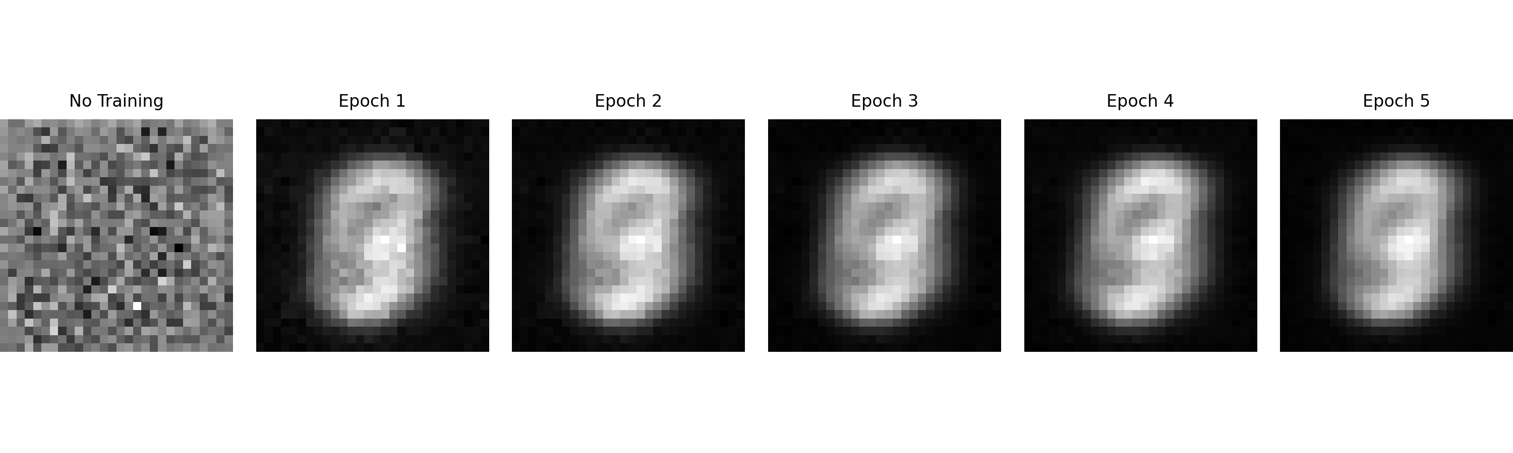
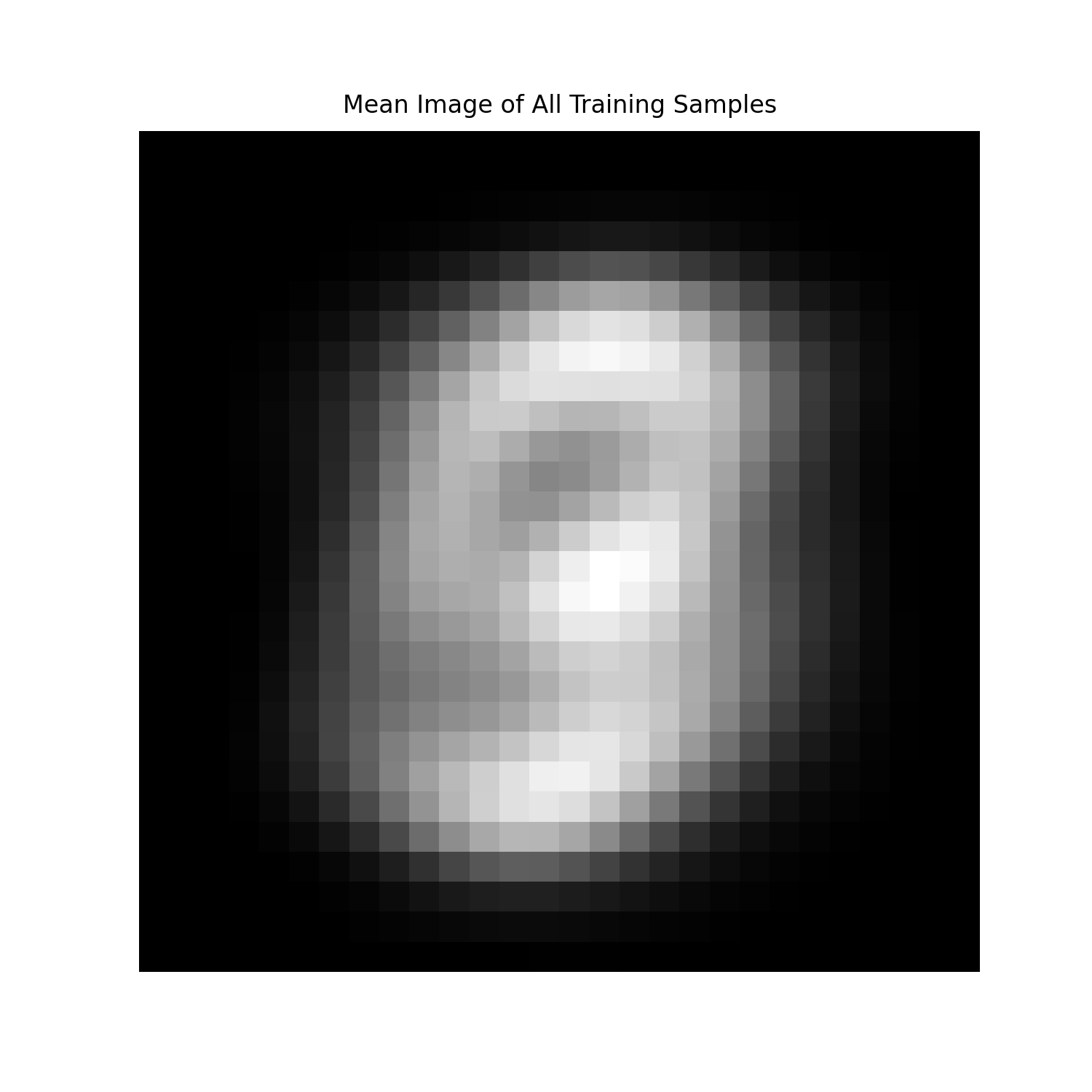
1.2.3 Denoising Pure Noise

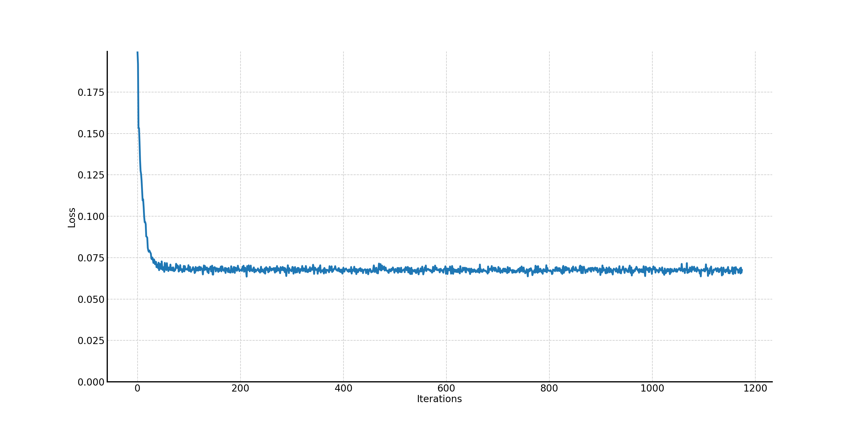
To make denoising a generative task, now we can denoise pure, random Gaussian noise. We can think of this as starting with a blank canvas \(z = \epsilon\), where \(\epsilon \sim \mathcal{N}\left(\mathbf{0}, \mathbf{I}\right)\), and denoising it to get a clean image \(x\). The training loss curve for this case is shown in Figure 34. Compared with Figure 31, the training loss curve with \(\sigma = 0.5\), we know that the training loss does not converge well. We sample some results on pure noise after 1 to 5 epochs, as shown in Figure 35. Figure 35 means that denoising pure, random Gaussian noise with one-step unconditonal UNet does not work. This is foreseeable because we choose MSE loss as the criterion, which means the model will learn the average image of the training set. To validate this idea, in Figure 36, we show the average image of all images in the training set, which is consistent with Figure 35 (epoch 5).

Part B.2: Training a Flow Matching Model

We just saw that one-step denoising does not work well for generative tasks. In this part, we will iteratively denoise the image with flow matching, specifically, the rectified flow.

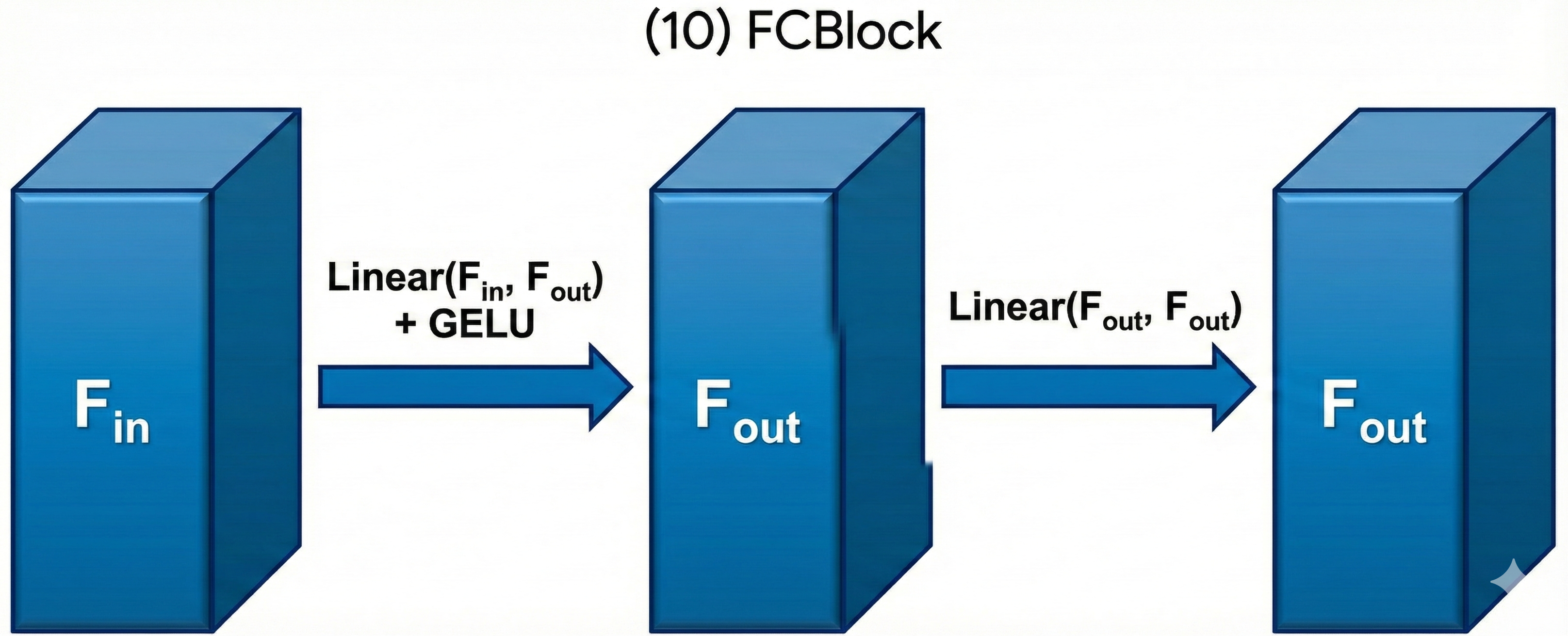
2.1 Adding Time Conditioning to UNet

We need a way to inject scalar \(t\) into our UNet model to condition it. There are many ways to do this. In this part, we use a fully-connected block (FCBlock) to project \(t\) on to \(2D\) dimensions, then concat it with the "Unflatten" and "UpBlock" module, as shown in Figure 37. FCBlock is actually a bunch of linear layers with activation functions, as shown in Figure 38. You can expand the time conditioned UNet architecture block to see the details.

We can embed \(t\) by following this pseudo code:

2.2 Training the UNet

The algorithm to train the time-conditioned UNet can be found below.

The model configuration for the time-conditioned UNet is shown in Table 2.

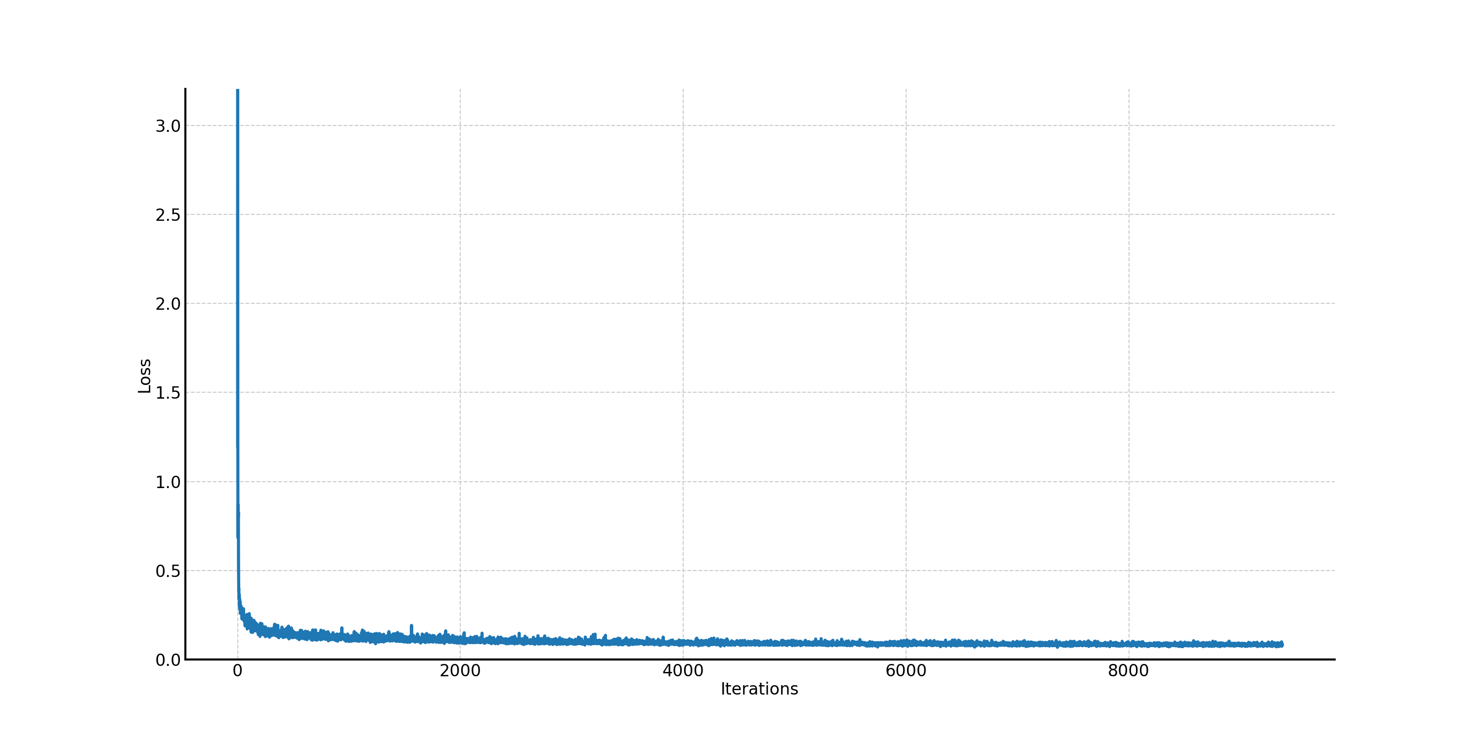
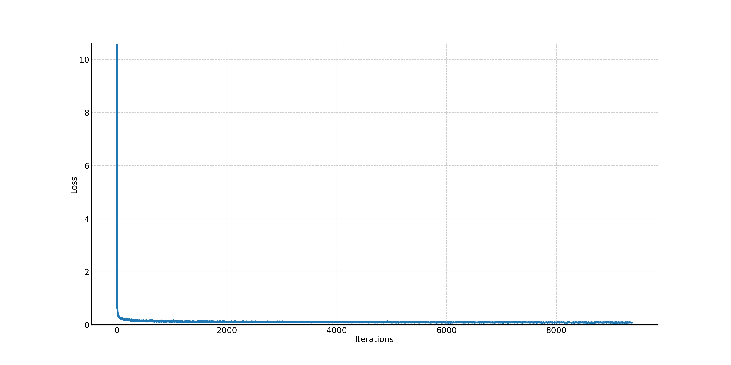
The corresponding training loss curve is shown in Figure 39.

2.3 Sampling from the UNet

We can now use the trained time-conditioned UNet for iterative denoising using the algorithm below.

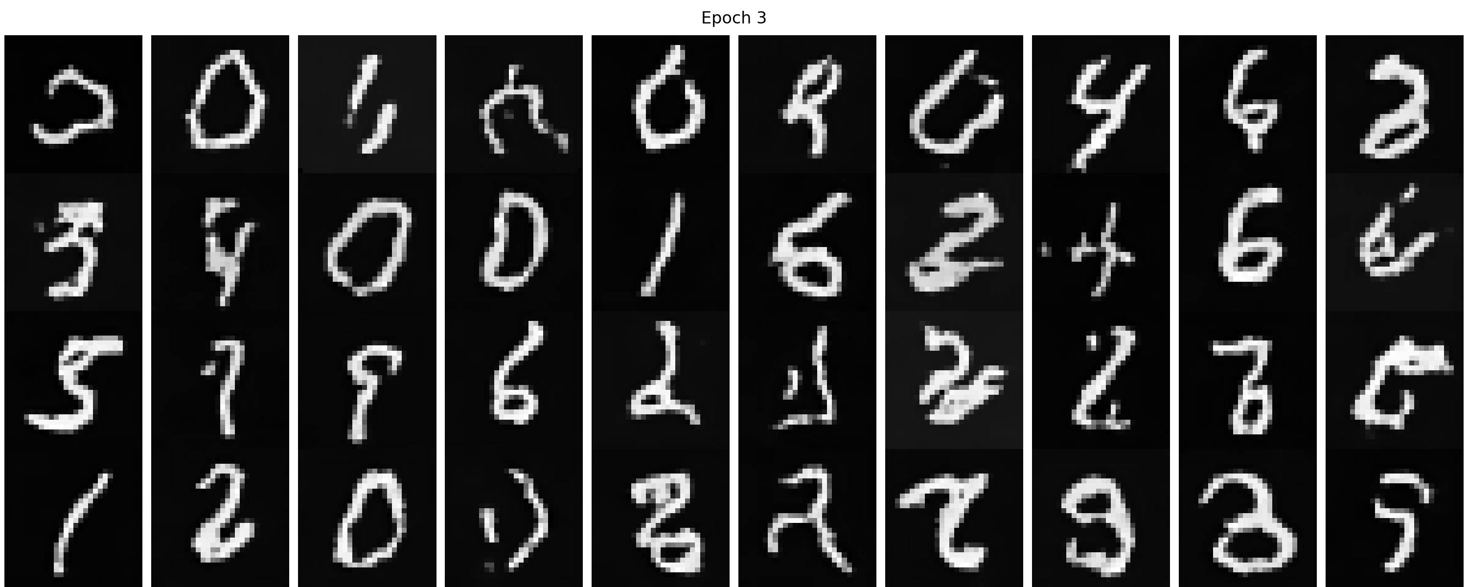
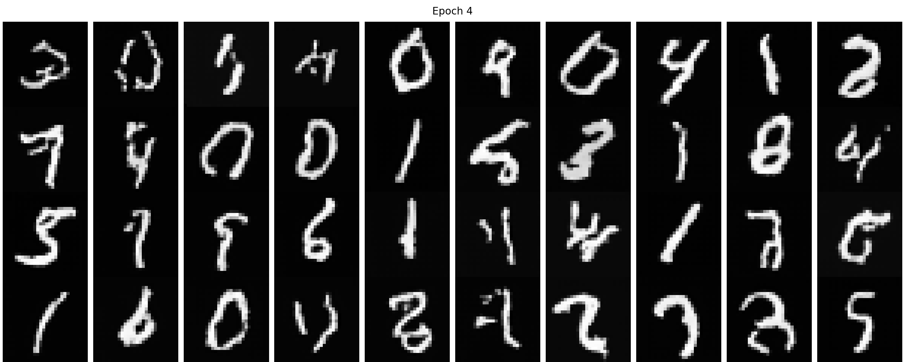
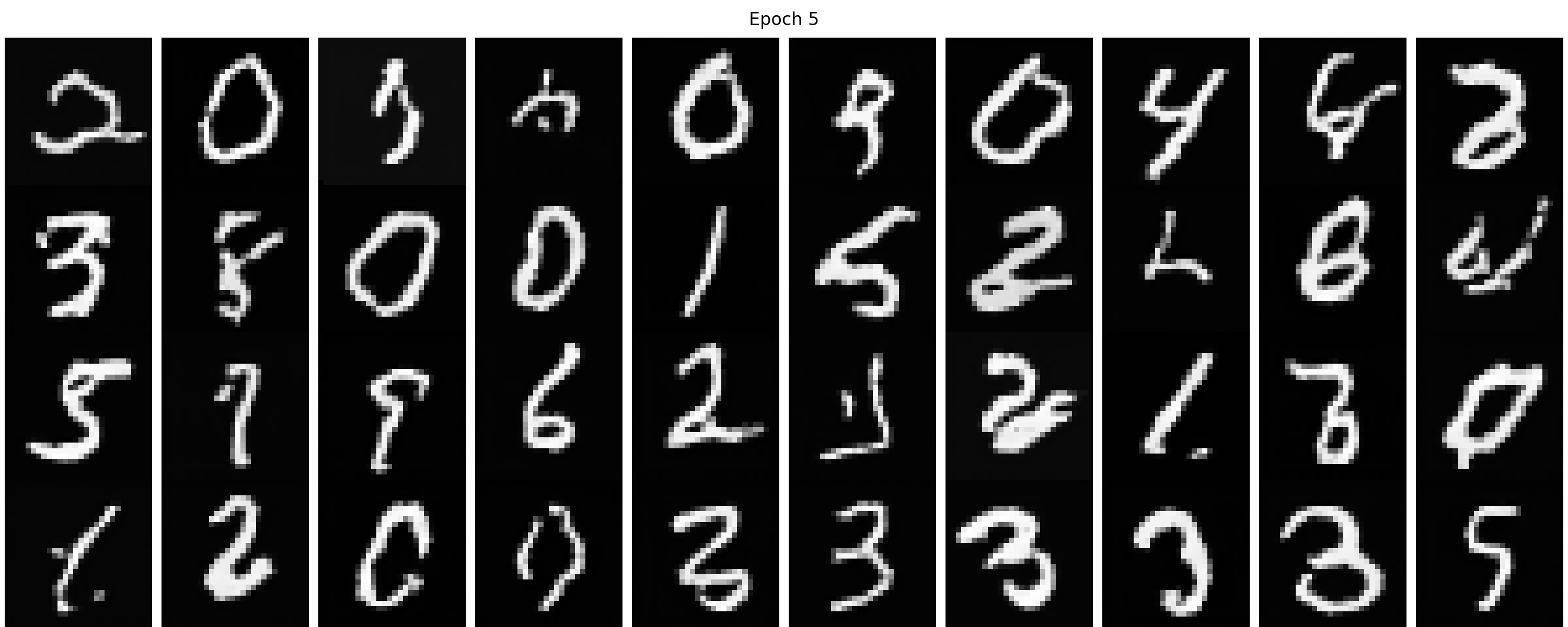
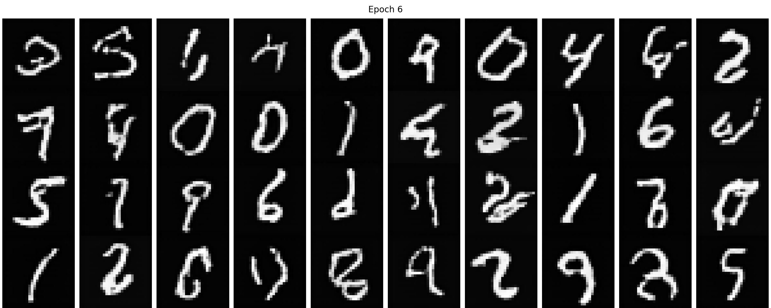
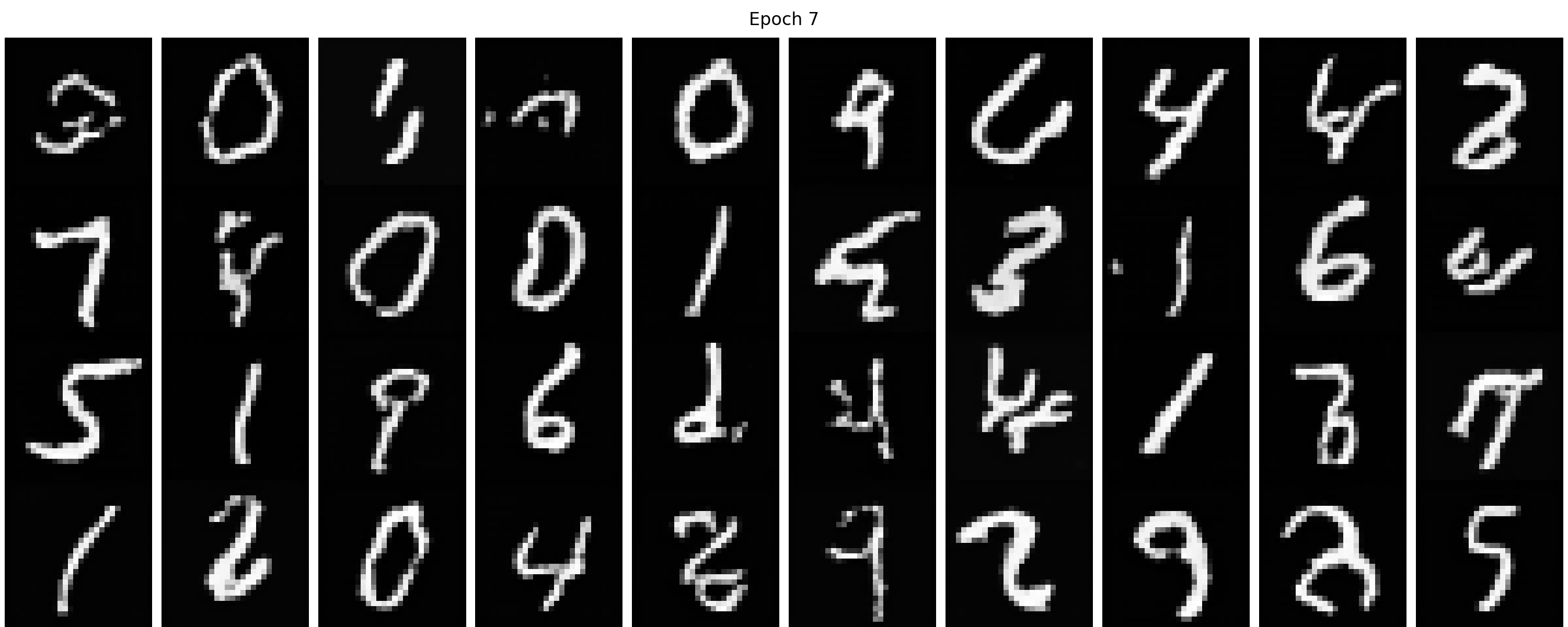
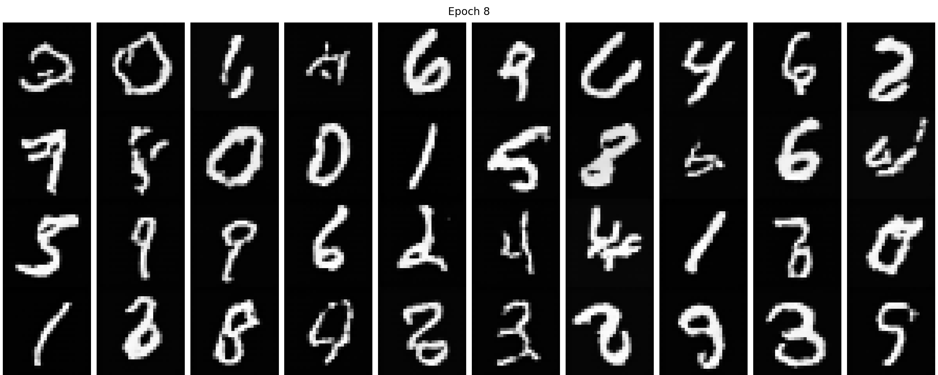
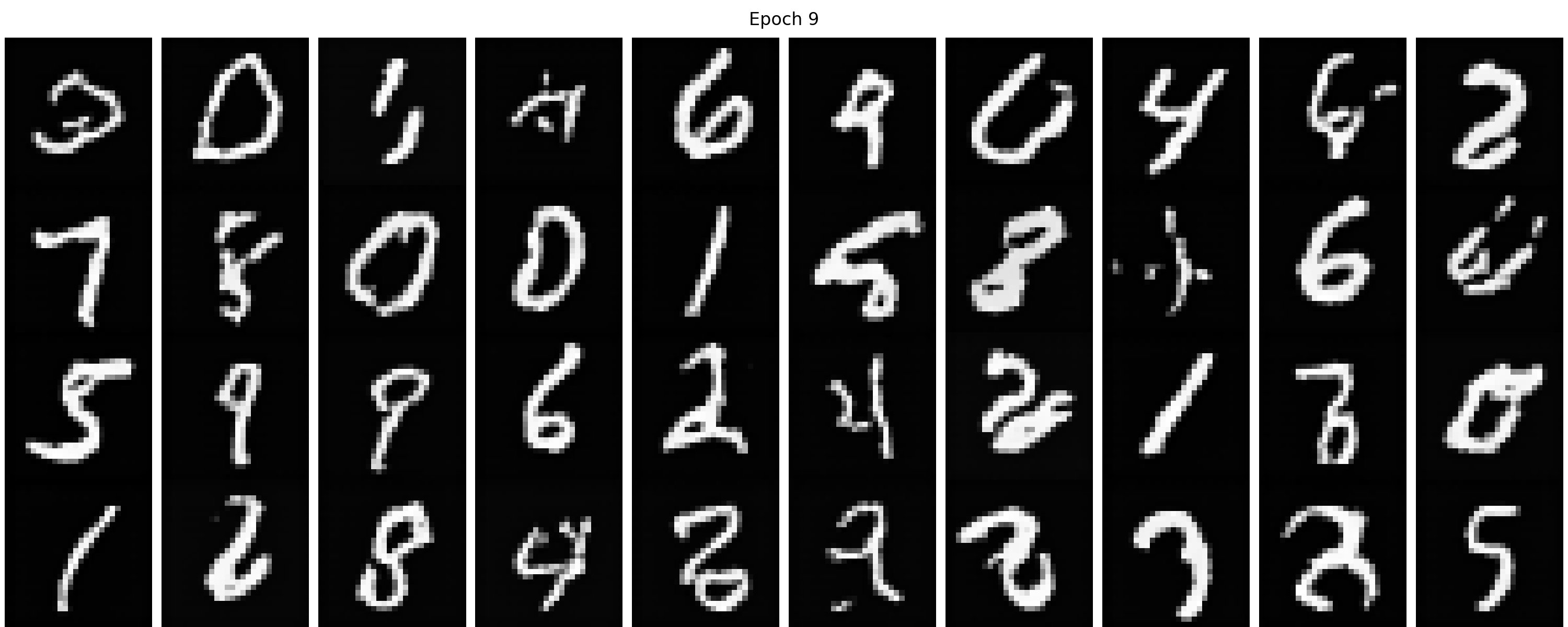
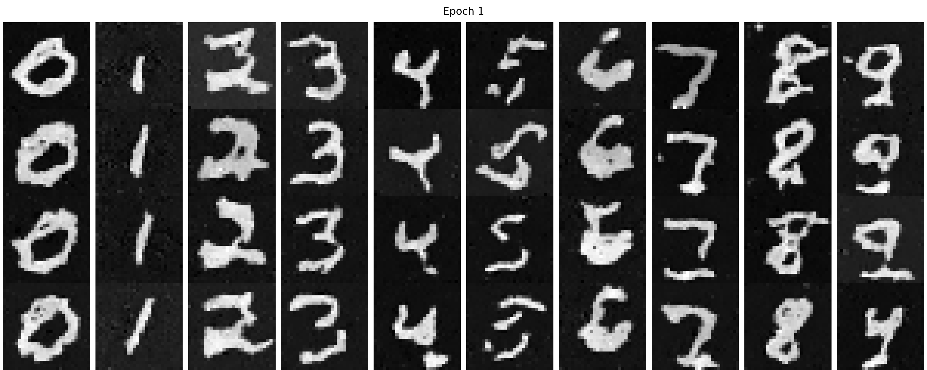
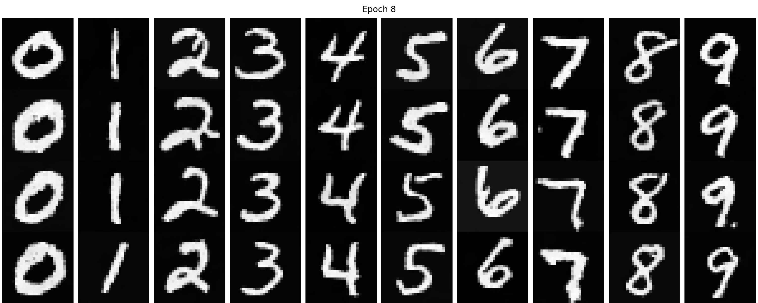
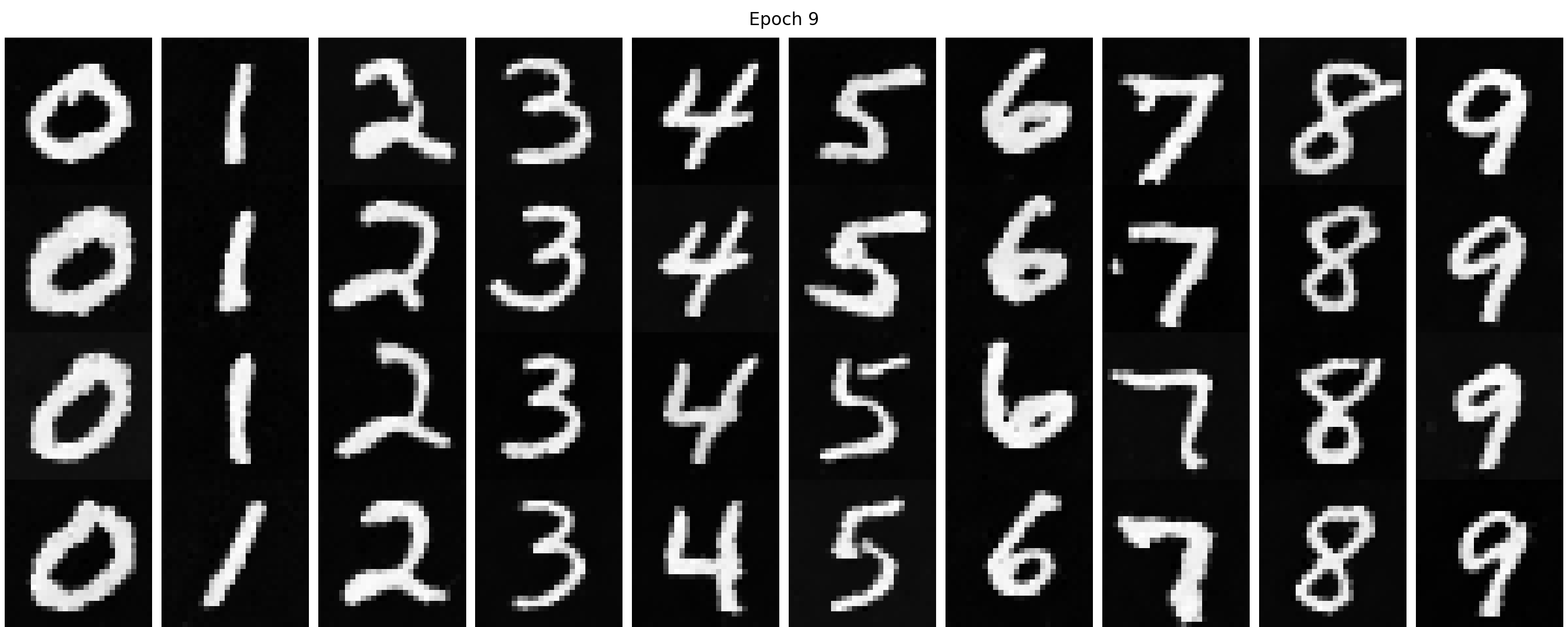
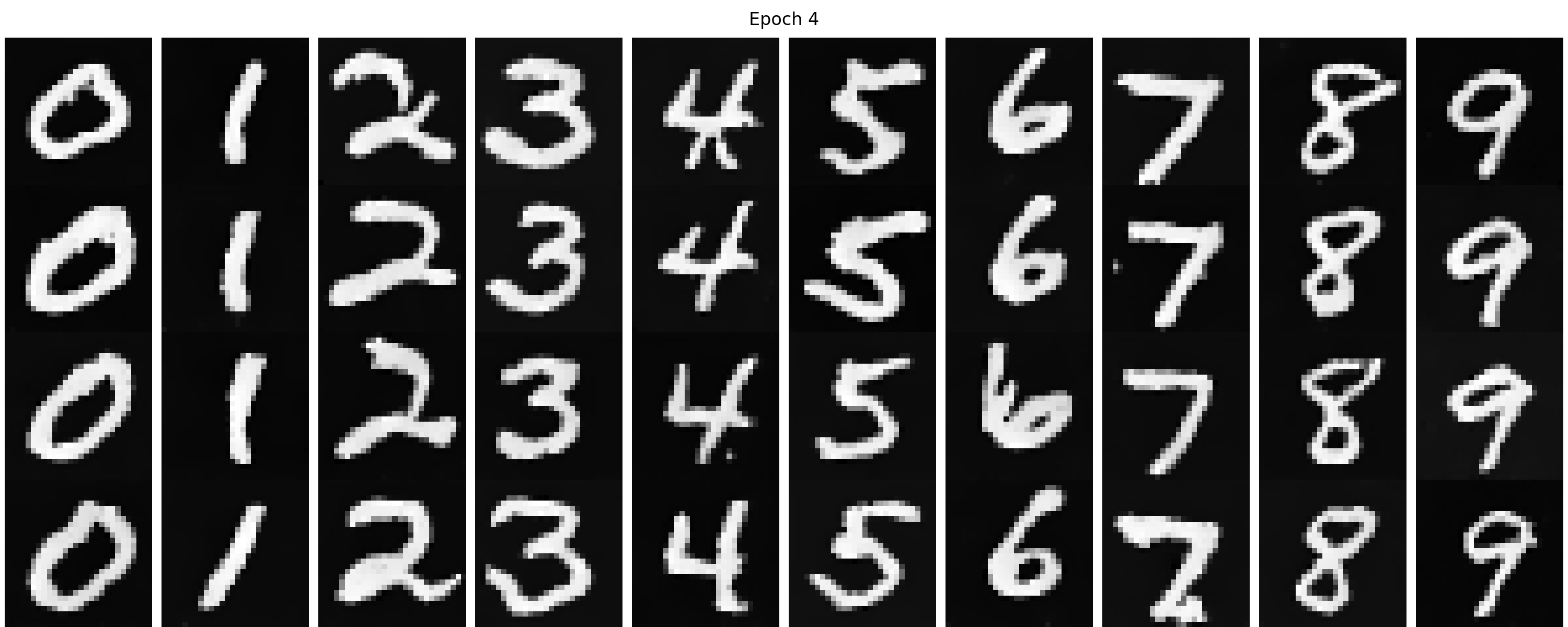
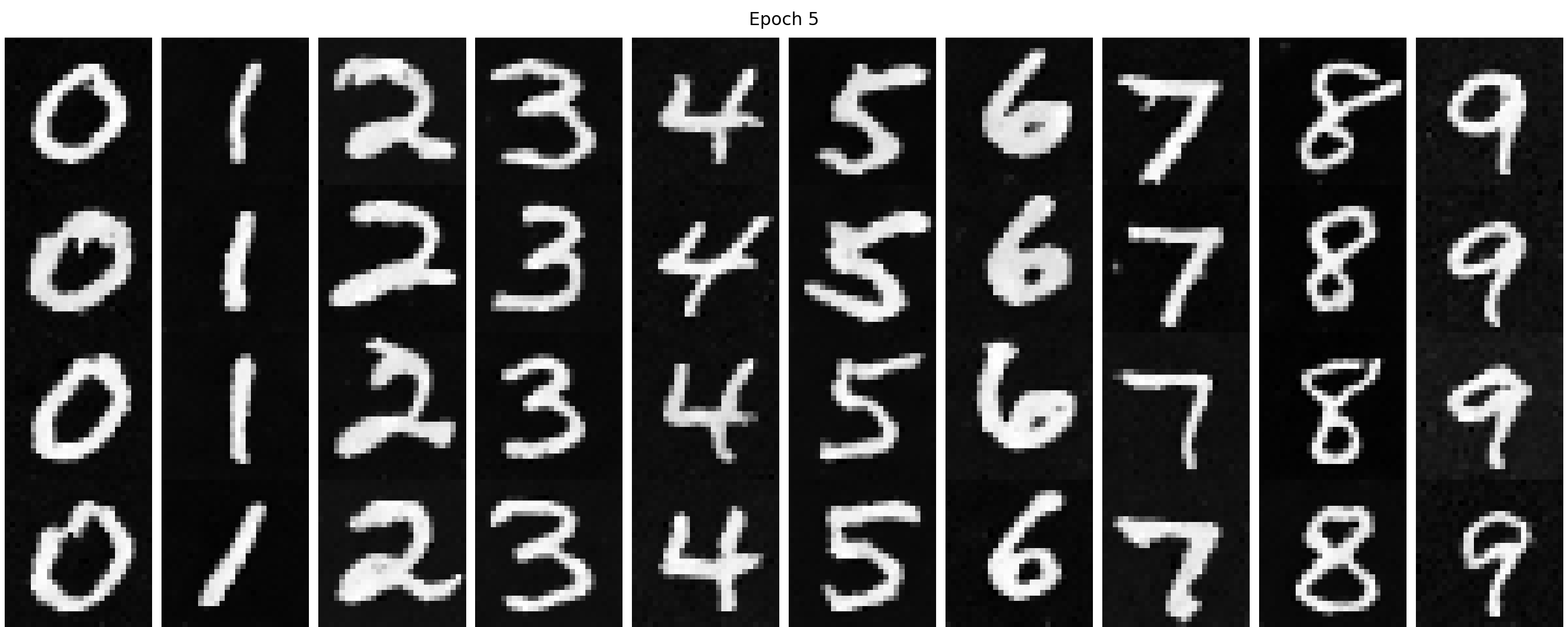
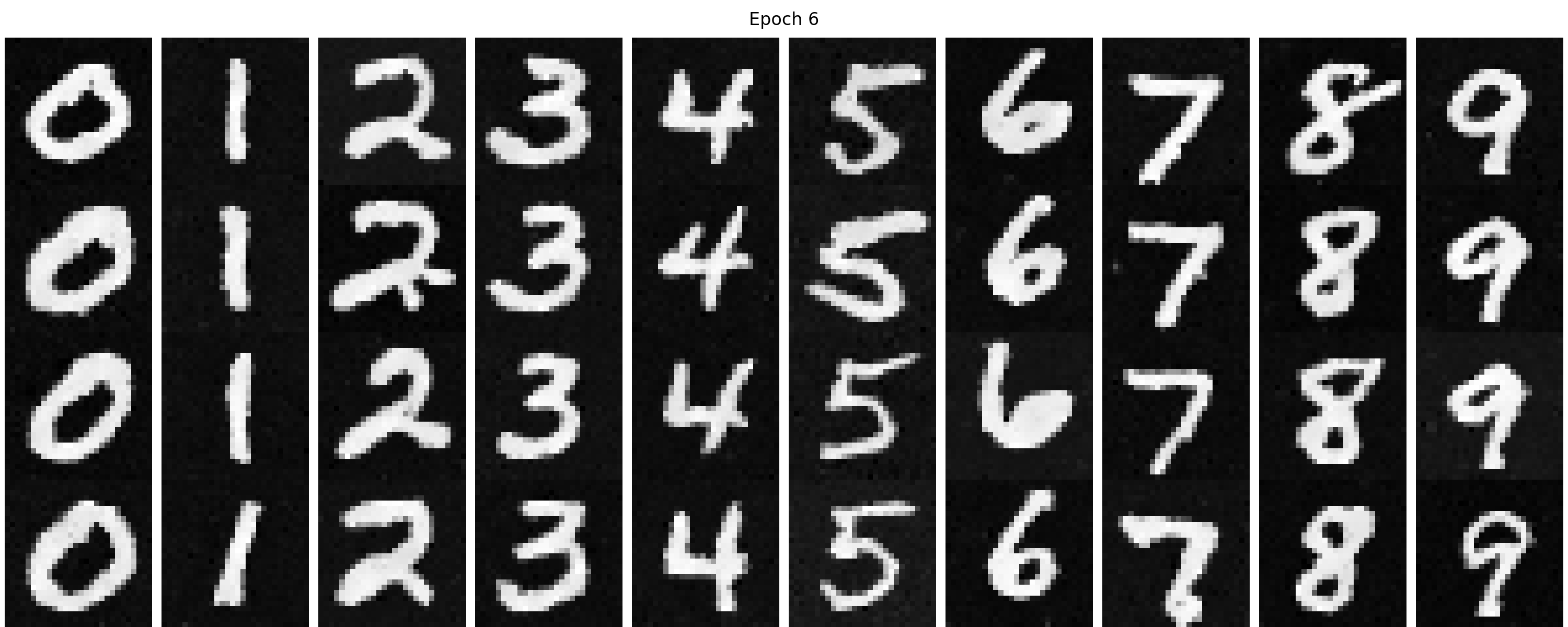
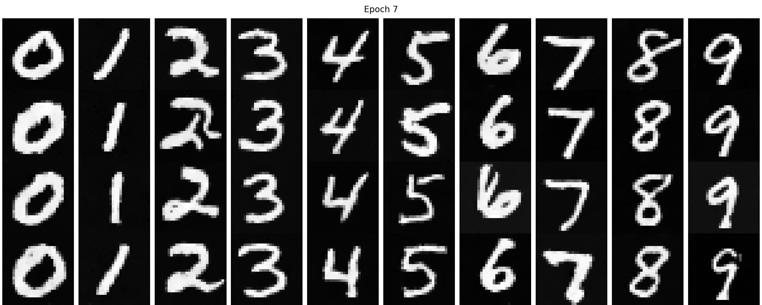
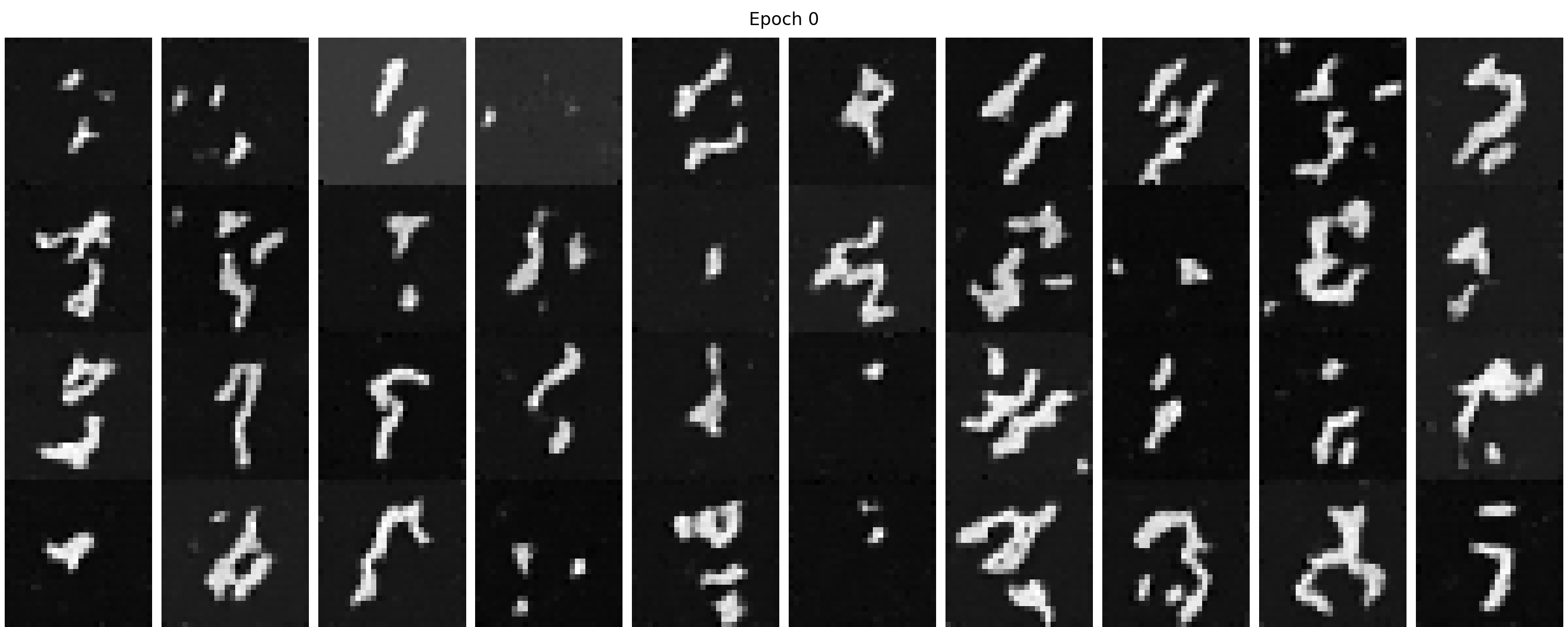
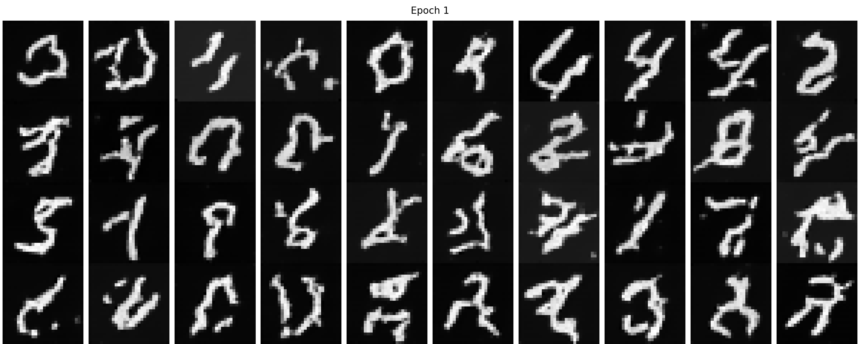
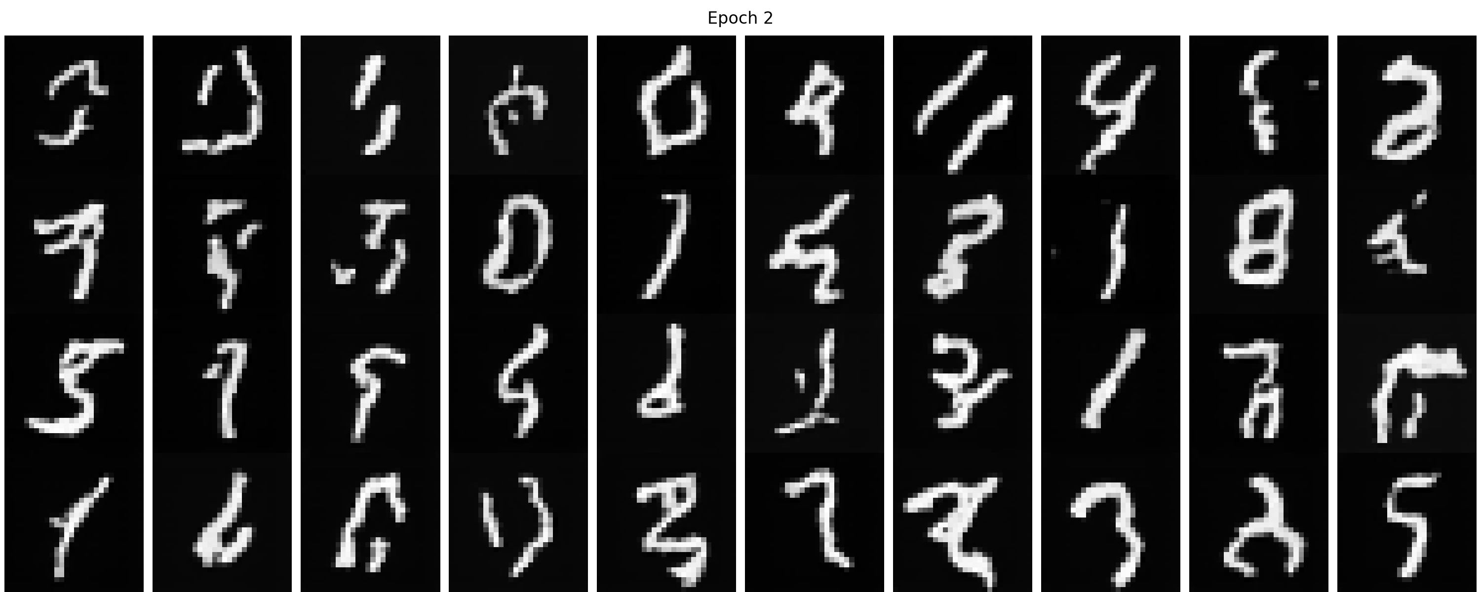
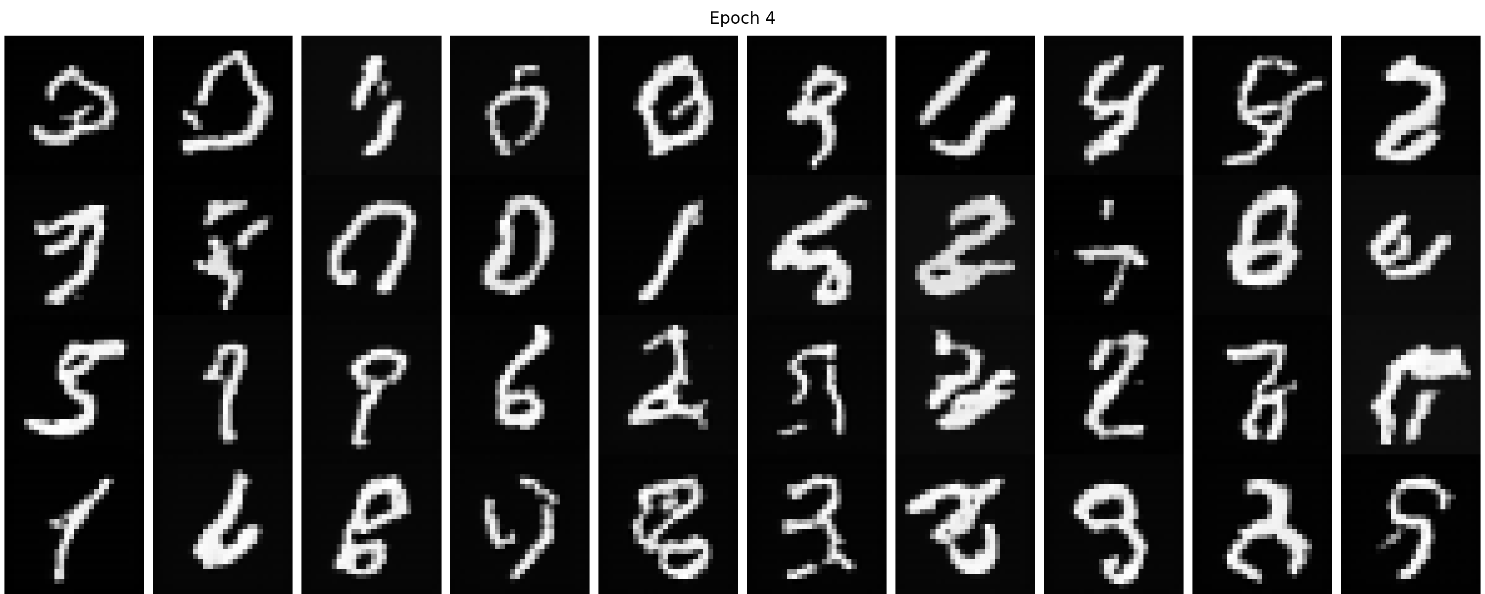
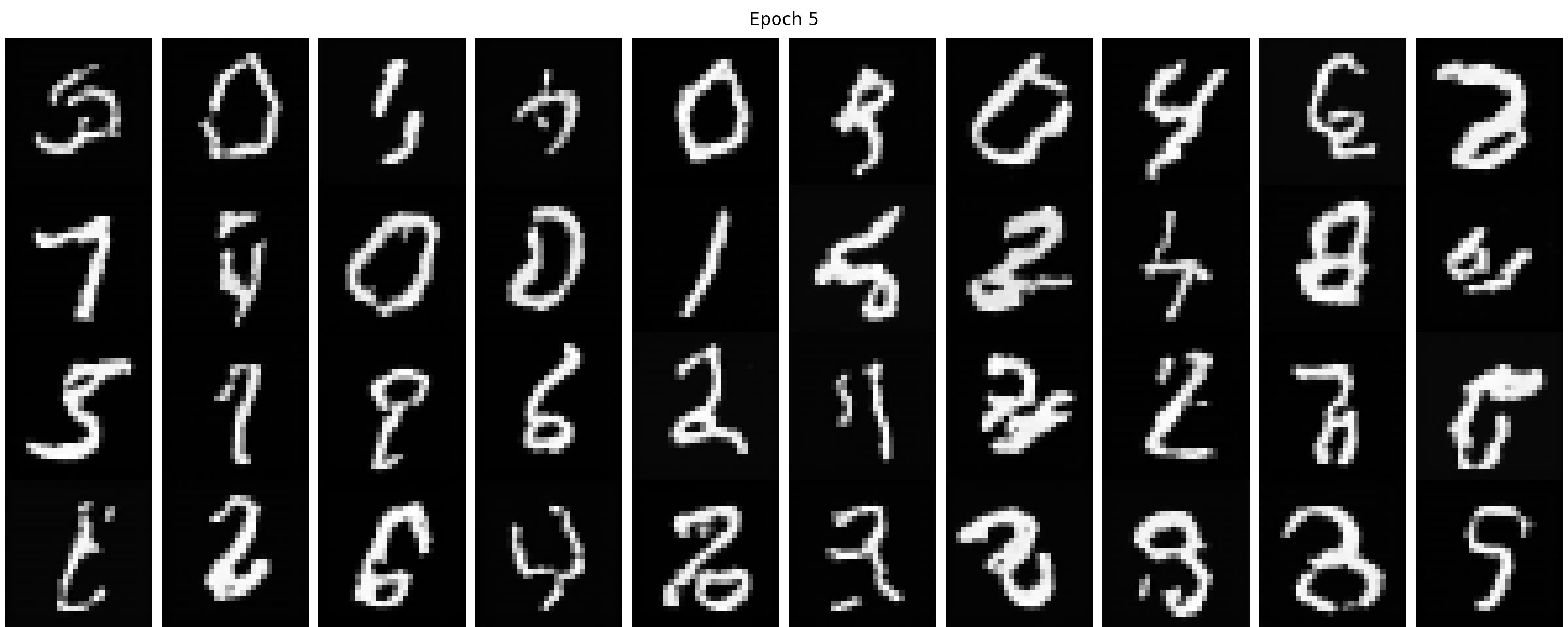
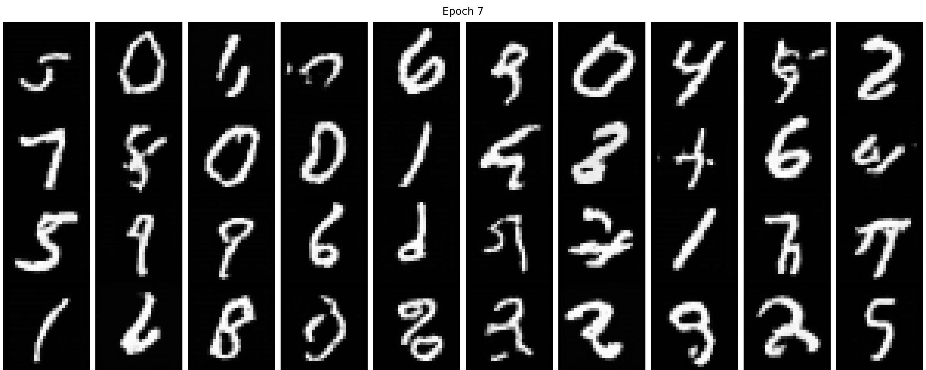
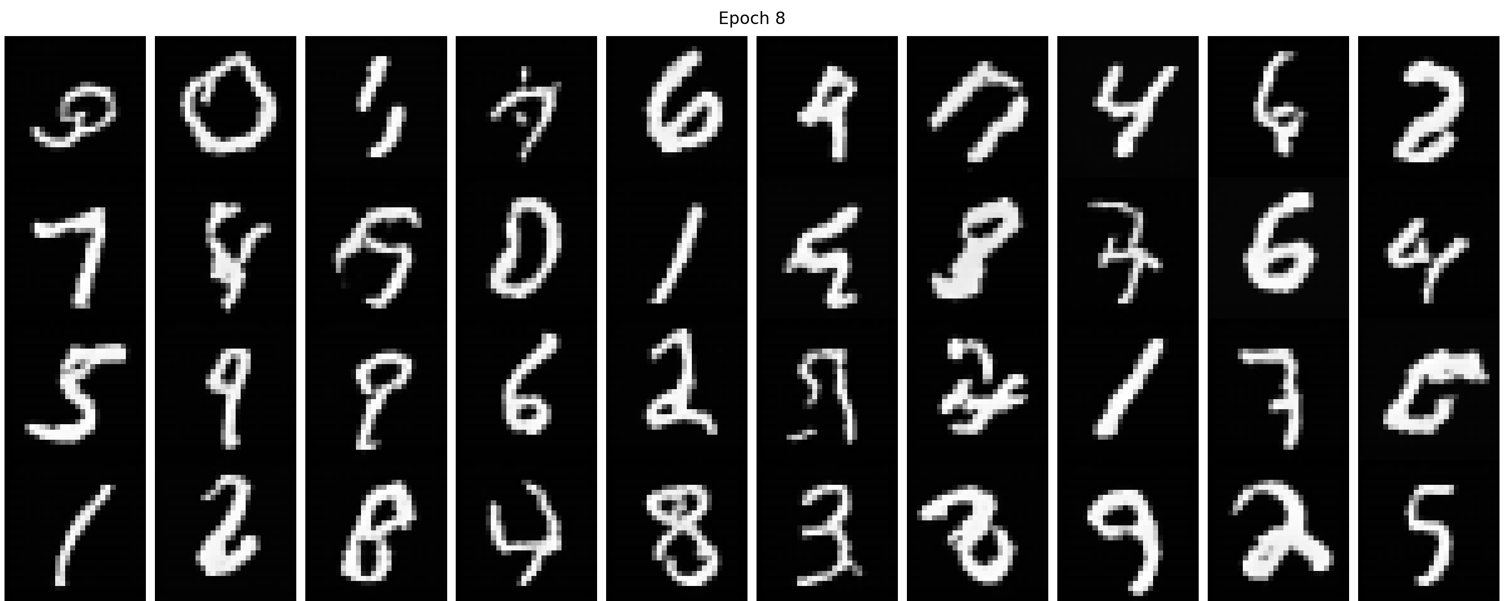
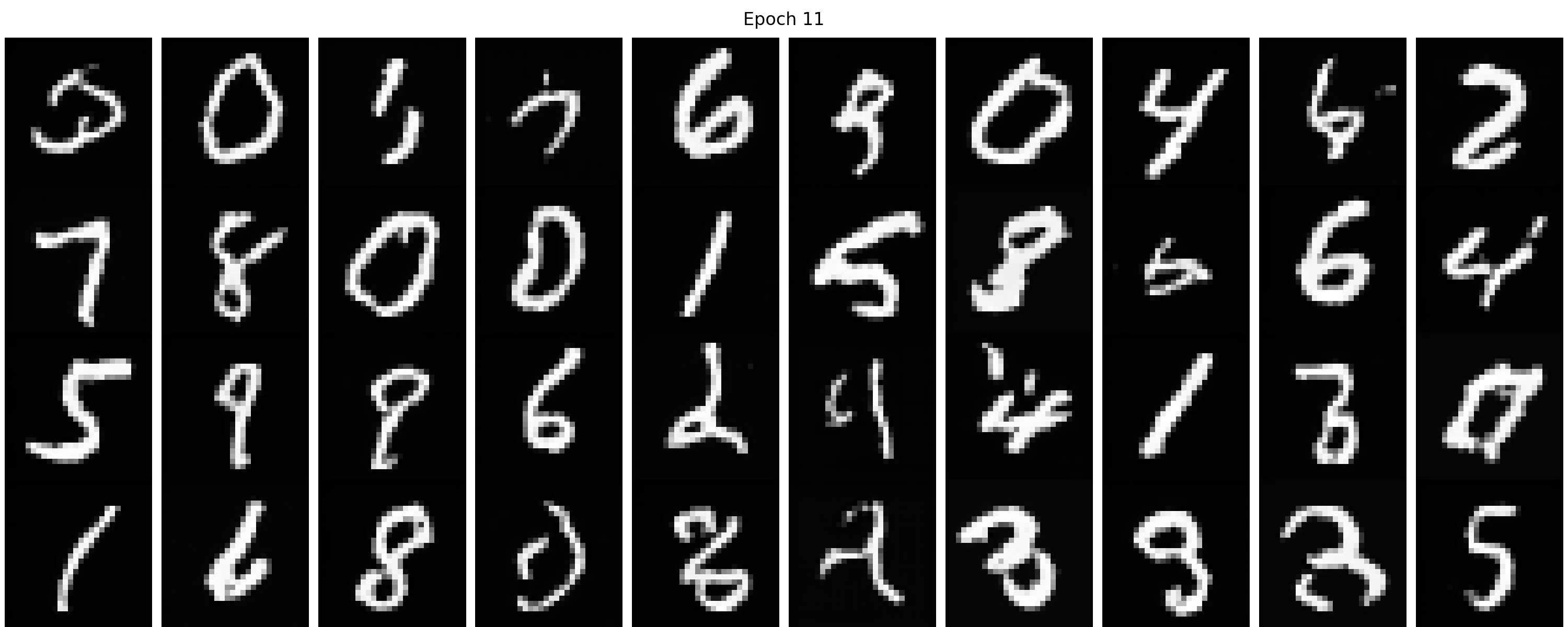
We show our sampling results from the time-conditioned UNet from 1 to 10 epochs in Figure 40. We can find with more training epochs, the results are gradually getting better. At the very beginning stage, say epoch 1, the generated image is vague and is hard to distinguish. With enough training, the image first becomes clearer; then we can gradually tell the digit in each image, though some of which are not like a normal digit. These results are expected because it is only time-conditioned but not class-conditioned, which means the denoiser tries to imitate randomly from the training set and does not know the specific digit to generate.

2.4 Adding Class-Conditioning to UNet

Now let's make it a class-conditioned UNet, which should be able to generate distinguishable digits according to the prompt. In this part, we make the class-conditioning vector \(c\) a one-hot vector instead of a single scalar because we still want our UNet to work without it being conditioned on the class (recall how classifier-free guidance works). To make the classifier-free guidance work, we implement dropout for 10% of the time, which means we set the one-hot vector \(c\) to be the zero vector. The details of how to embed \(t\) and \(c\) can be found below. You can also expand the class-conditioned UNet architecture block to see the details.

2.5 Training the UNet

The algorithm to train the class-conditioned UNet can be found below.

The model configuration for the class-conditioned UNet is shown in Table 3.

The corresponding training loss curve is shown in Figure 41.

2.6 Sampling from the UNet

Now we will sample with class-conditioning and use classifier-free guidance with \(\gamma = 5.0\). The algorithm is shown in Algorithm 4.

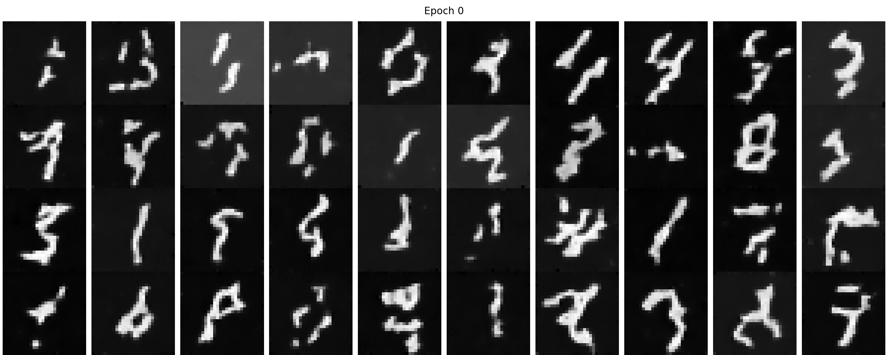
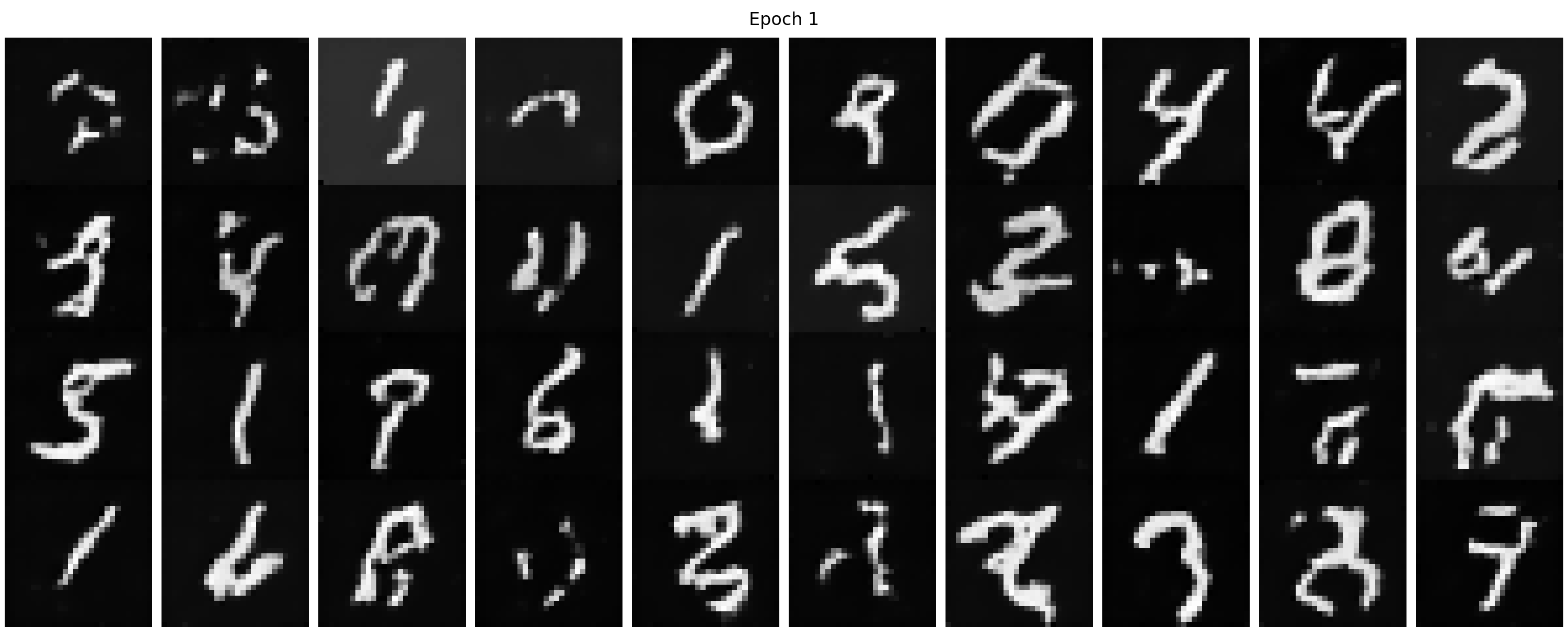
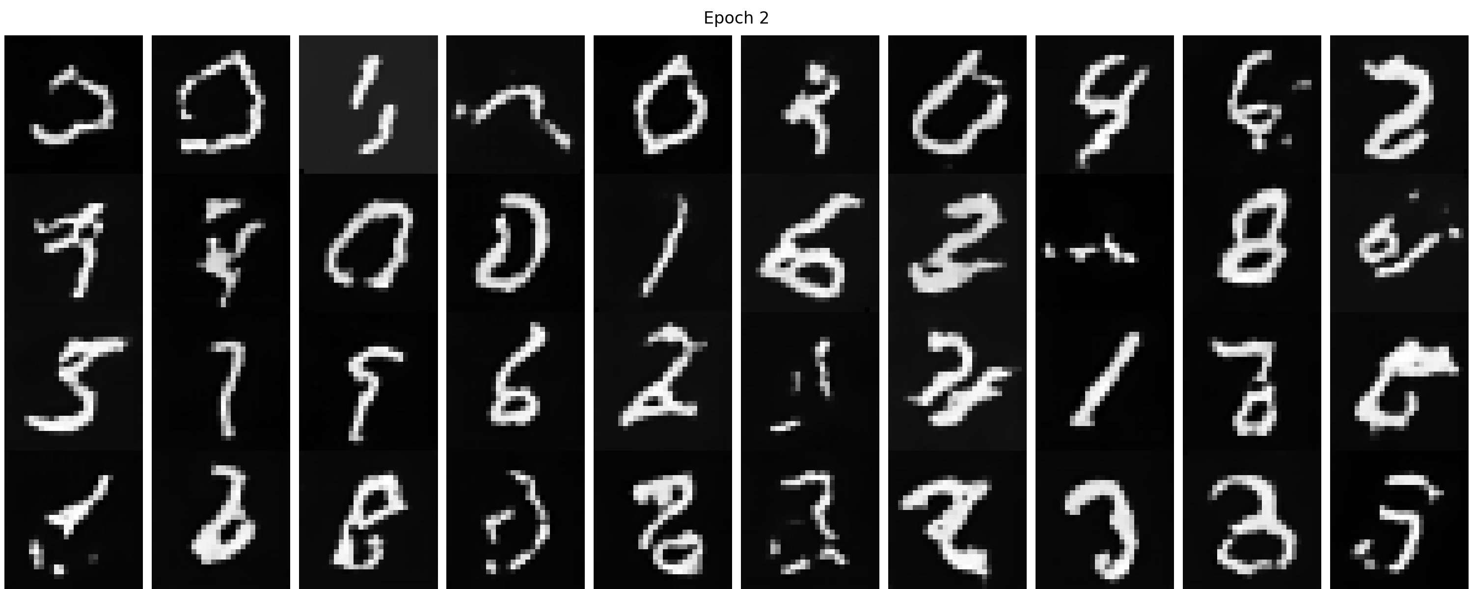
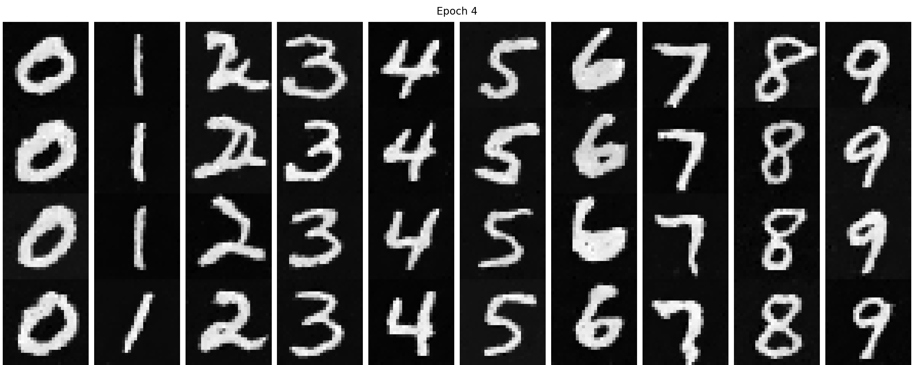
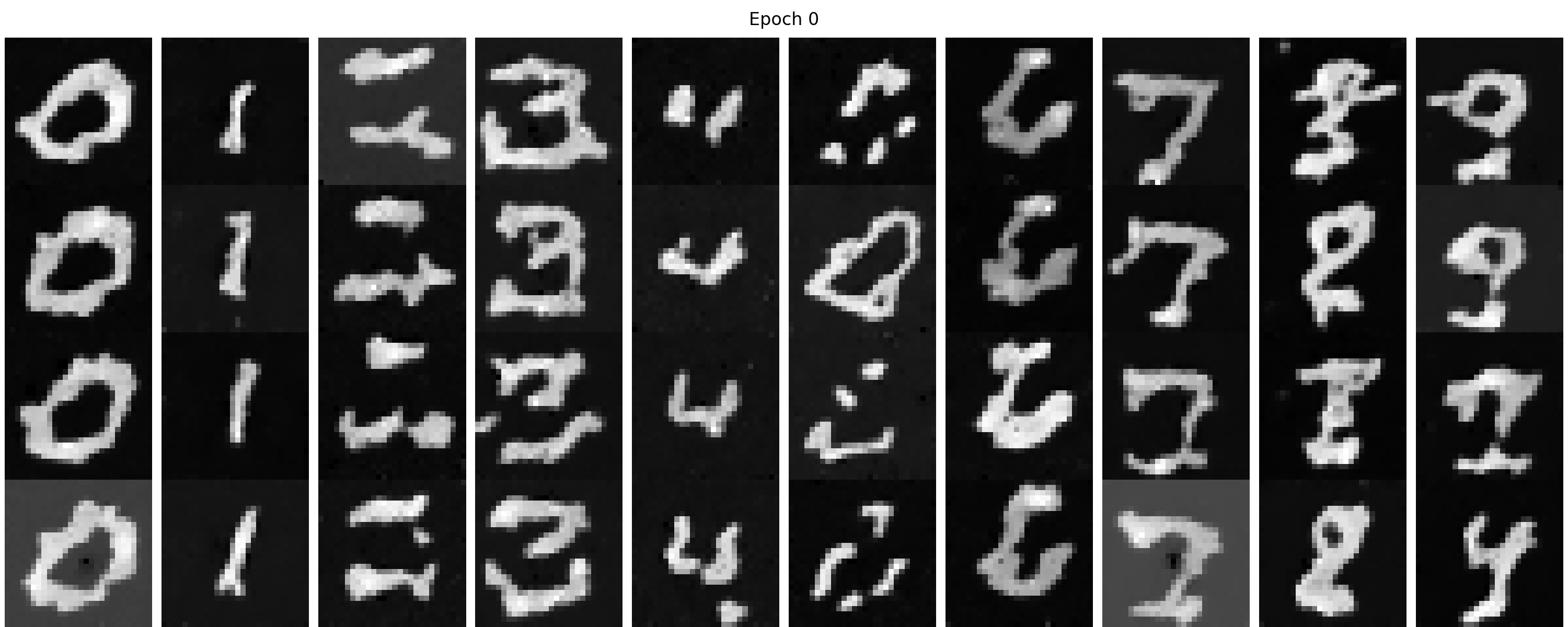
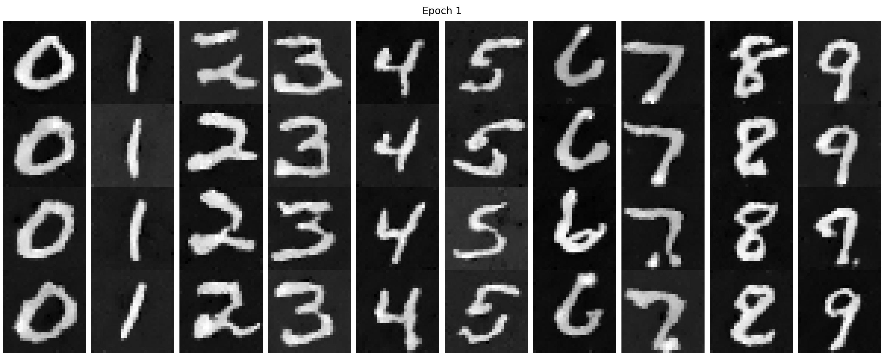
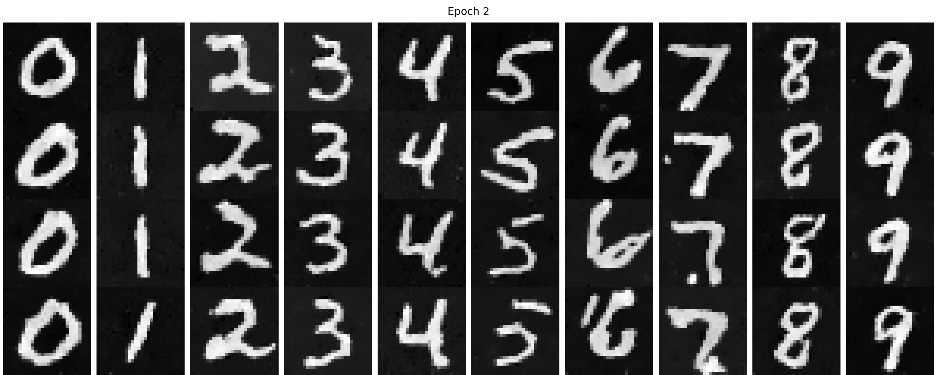
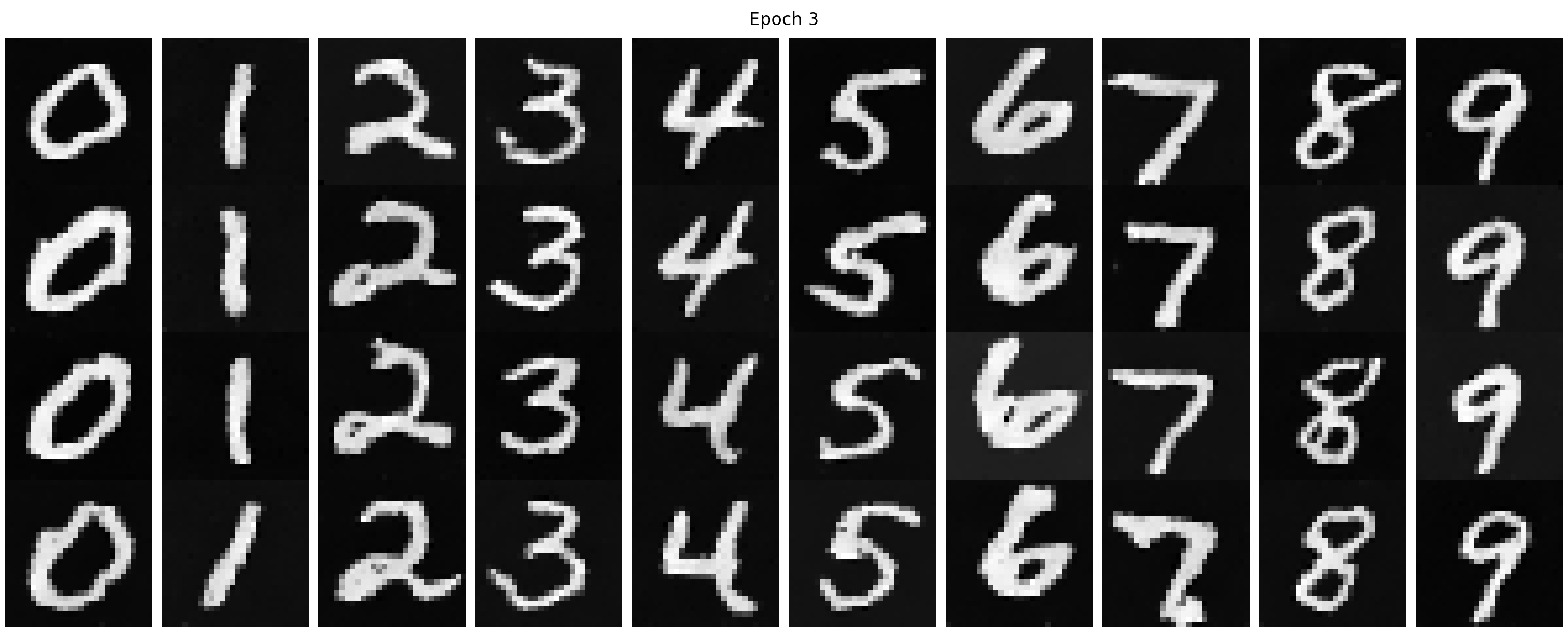
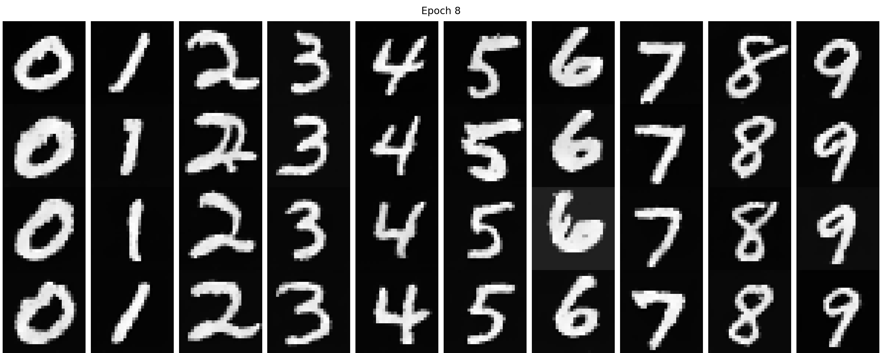
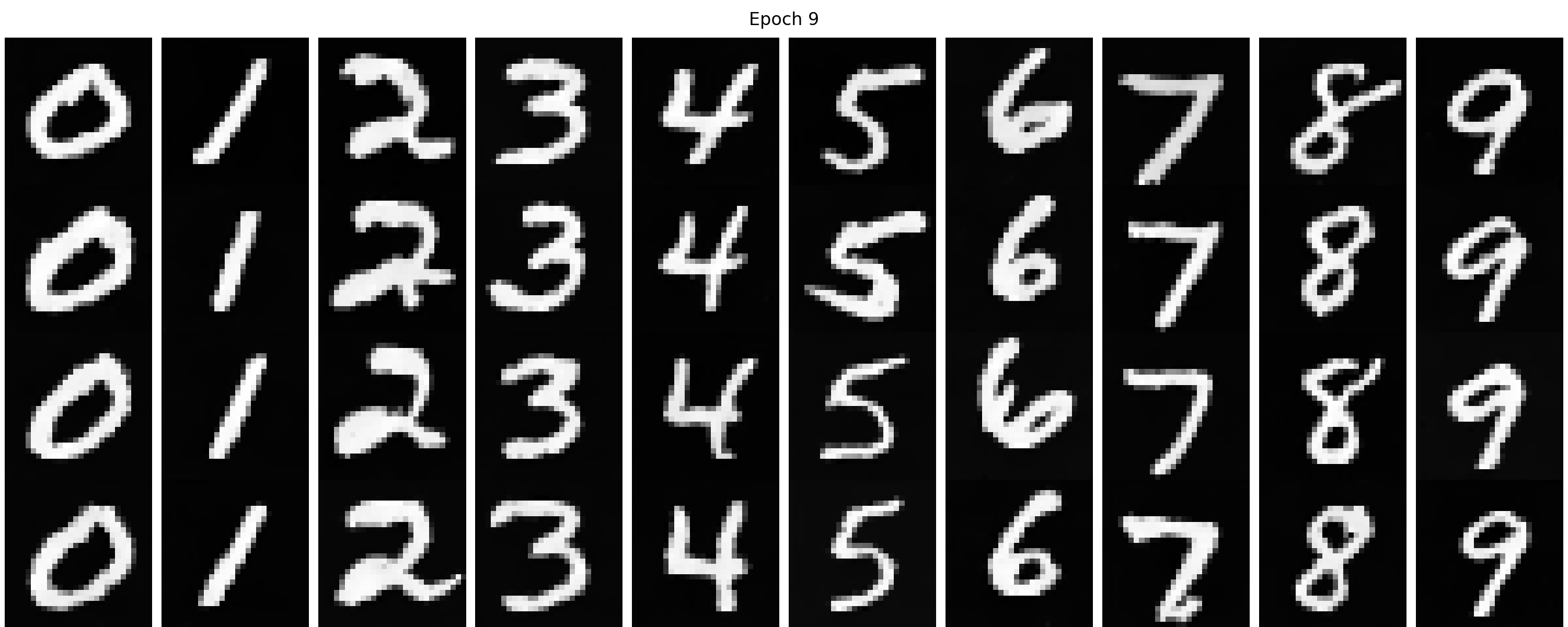
Figure 42 shows the sampling results from the class-conditioned UNet from 1 to 10 epochs. We can find that the denoising capacity becomes better with more training epochs. Compared with the time-conditioned UNet, the digit is more distinguishable and we can guide the generation, which is preferable.

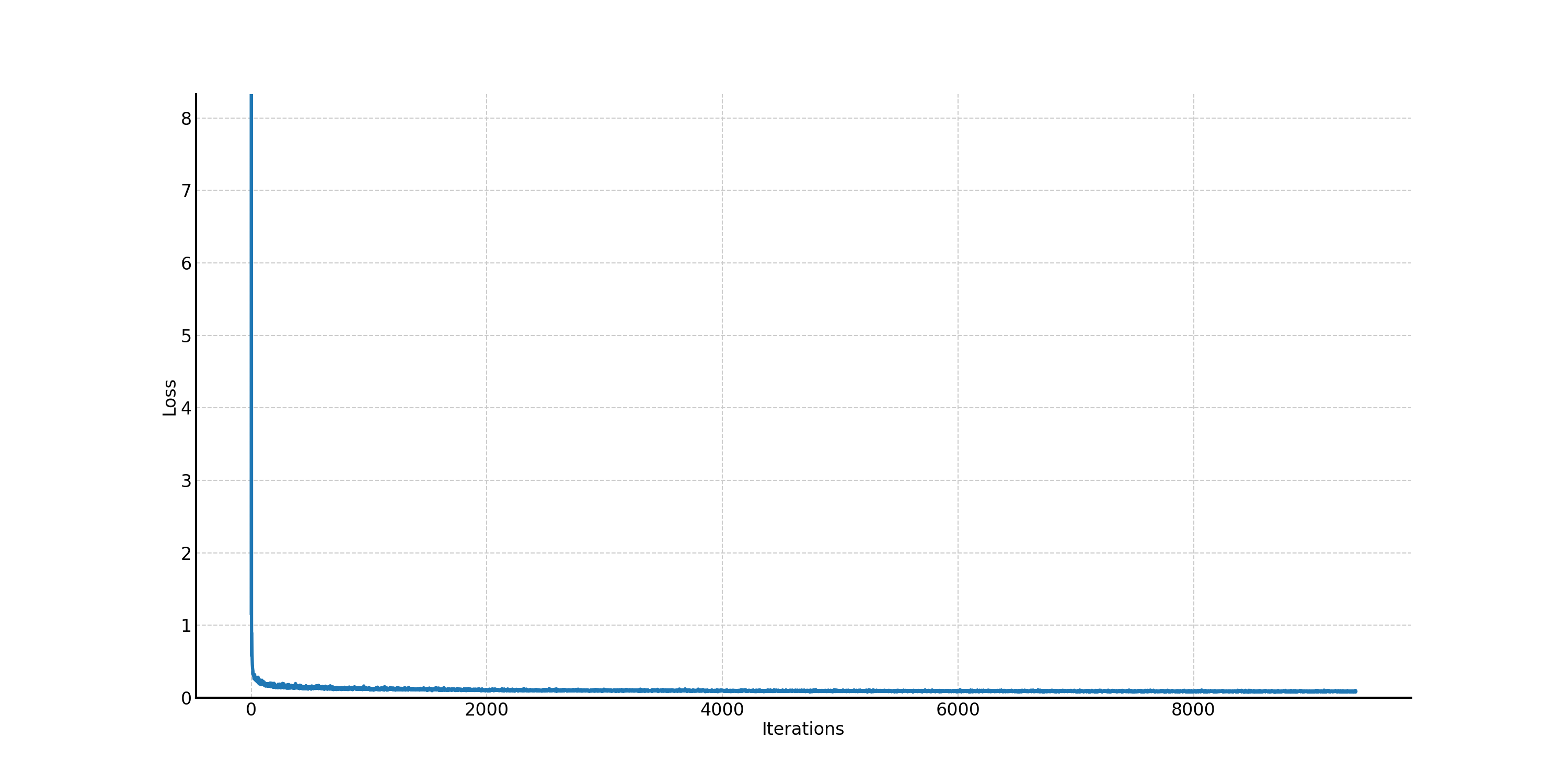
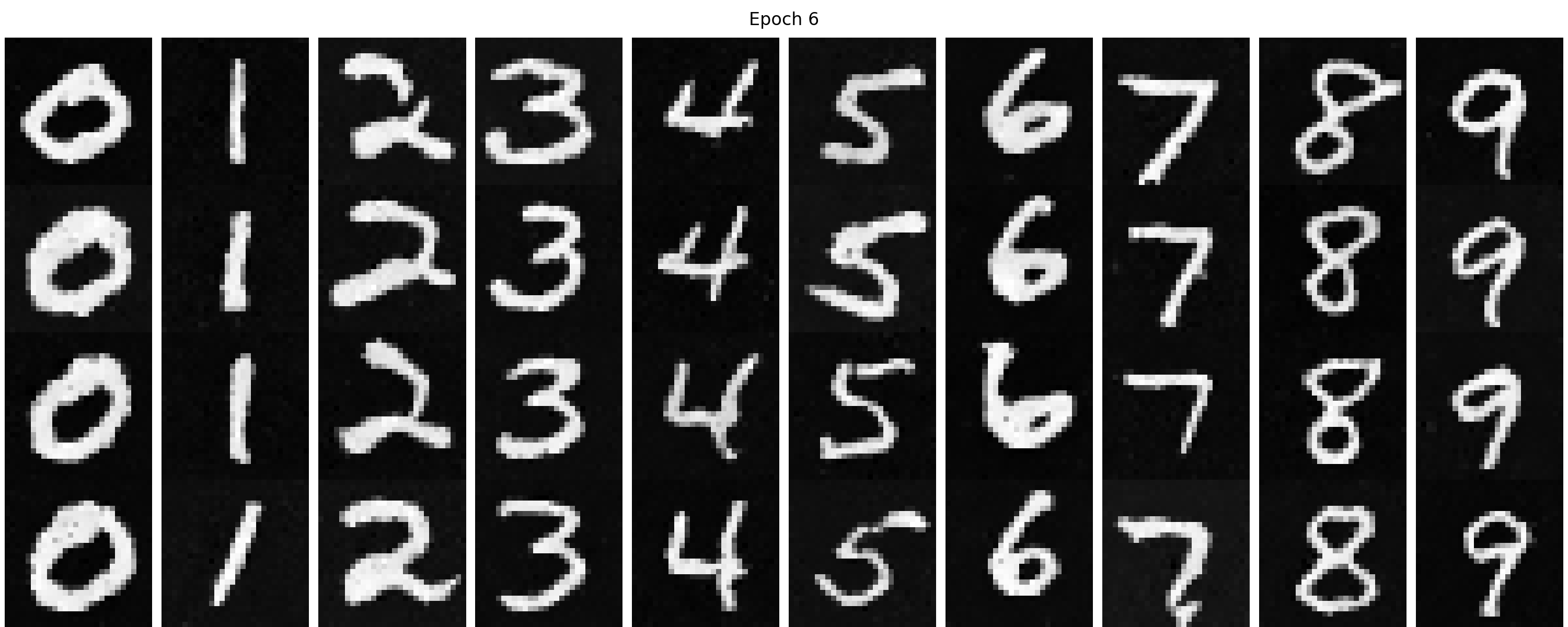
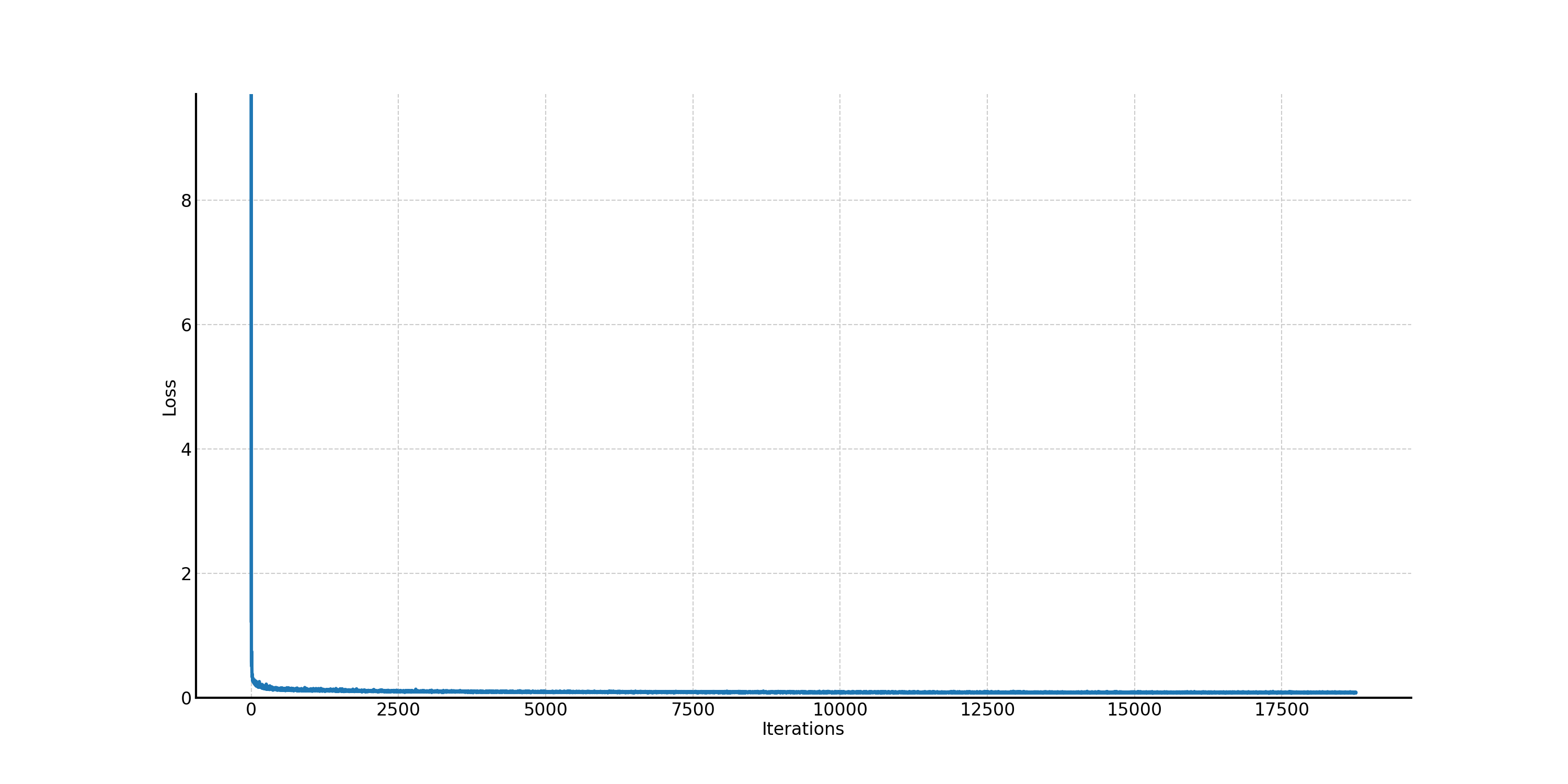
Now let's try to remove the learning rate scheduler to see how it affects the training and sampling results. We employ the same training settings as before except removing the learning rate scheduler. The training loss curve is shown in Figure 43, where you can see the training loss is surprisingly, nearly the same as before. It means that the flow matching model is very robust to the learning rate choice (at least in this simple experiment). The sampling results are similar to before as well, as shown in

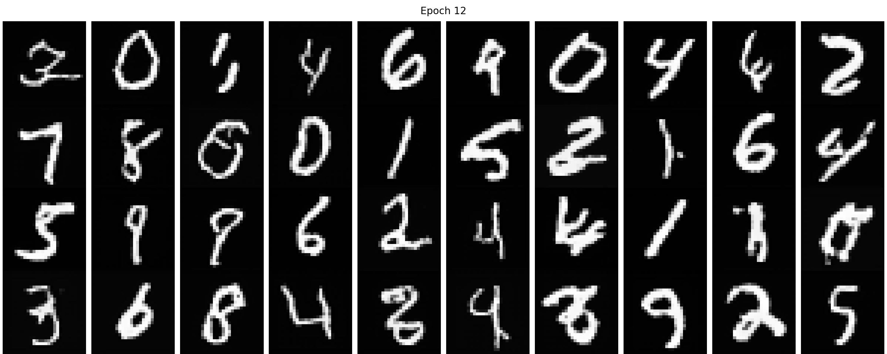
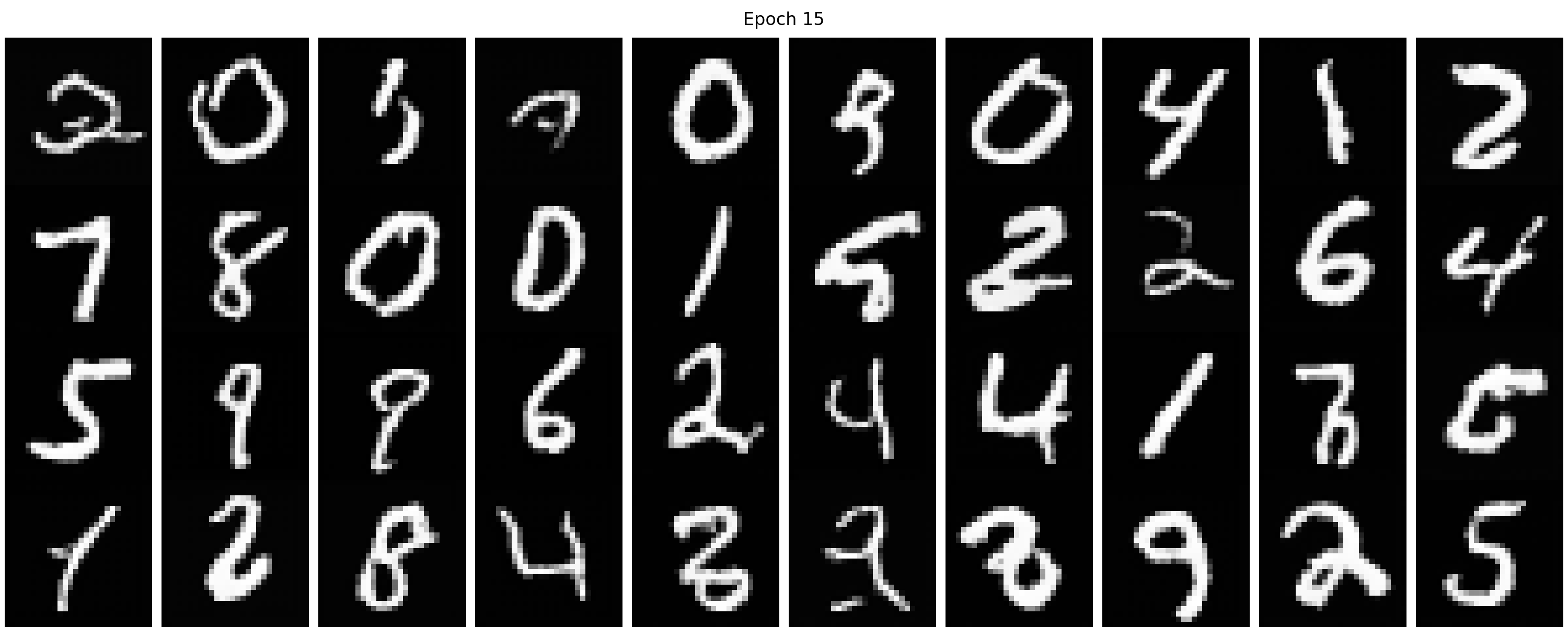
Part B.3: A Better Time-conditioned only UNet

In our previous time-conditioned only UNet experiment, we found that the generated images are not perfect, though most of them can be recognized as digits. Typically, the time-condtioned only UNet cannot surpass the class-conditioned UNet. However, we can definitely make it better than before by tuning the model architecture and training hyperparameters. In this part, we will show you one possible way to improve the time-conditioned only UNet. The model configuration for the improved time-conditioned UNet is shown in Table 4.

The corresponding training loss curve is shown in Figure 44, where the training loss (0.078) is lower than before (0.091), indicating a better model fit.

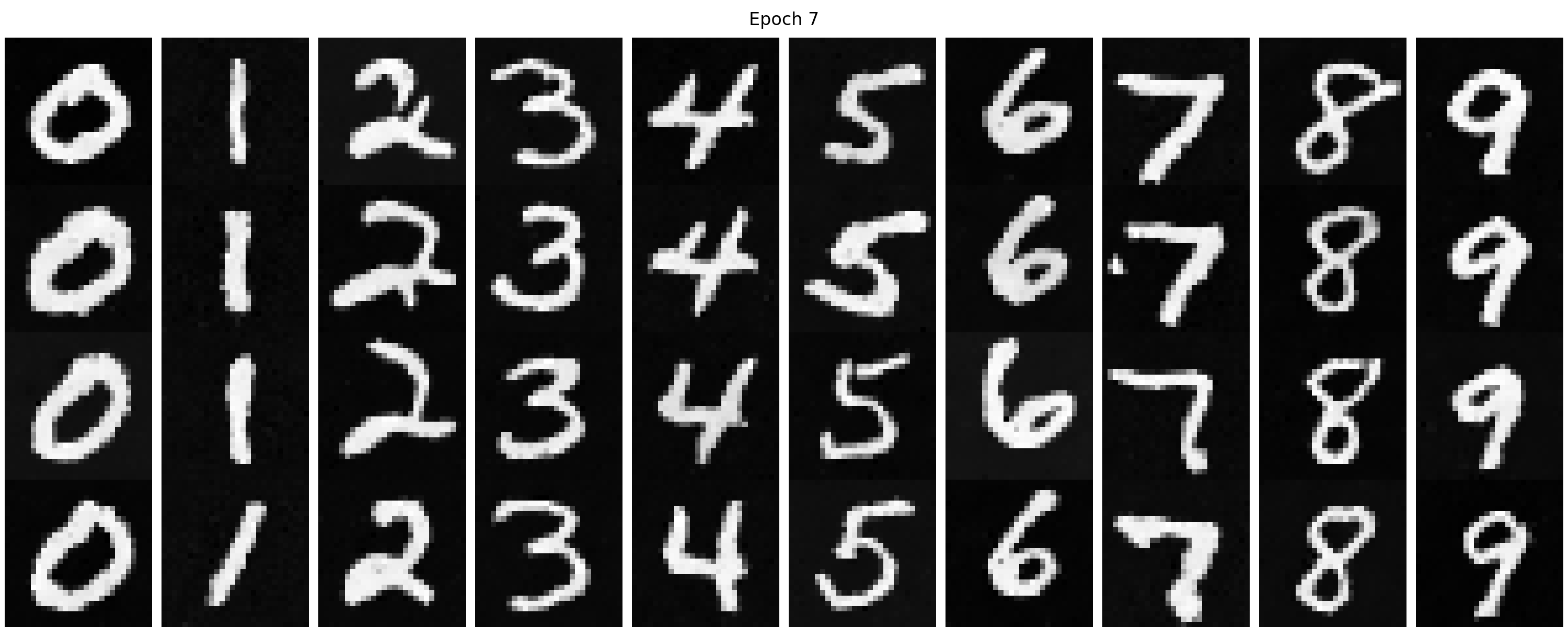
Figure 45 shows the sampling results from the improved time-conditioned UNet from 1 to 20 epochs. We can find that the denoising capacity becomes better with more training epochs. Compared with the previous time-conditioned UNet, the digit is more distinguishable and some of them are even comparable to the class-conditioned UNet results.